Chapter Contents

Previous

Next

Example 20.3: Working with Unequal Subgroup Sample Sizes

This example contains measurements from the metal clip manufacturing process (introduced in "Creating EWMA Charts from Raw Data" ). The following statements create a SAS data set named CLIPS4, which contains additional clip gap measurements taken on a daily basis:

   data clips4;
      input day @;
      length dayc $2.;
      informat day ddmmyy8.;
      format   day date5.;
      dayc=put(day,date5.);
      dayc=substr(dayc,1,2);
      do i=1 to 5;
         input gap @;
         output;
         end;
      drop i;
      label dayc='April';
   datalines;
    1/4/86  14.93  14.65  14.87  15.11  15.18
    2/4/86  15.06  14.95  14.91  15.14  15.41
    3/4/86  14.90  14.90  14.96  15.26  15.18
    4/4/86  15.25  14.57  15.33  15.38  14.89
    7/4/86  14.68  14.63  14.72  15.32  14.86
    8/4/86  14.48  14.88  14.98  14.74  15.48
    9/4/86  14.99  15.16  15.02  15.53  14.66
   10/4/86  14.88  15.44  15.04  15.10  14.89
   11/4/86  15.14  15.33  14.75  15.23  14.64
   14/4/86  15.46  15.30  14.92  14.58  14.68
   15/4/86  15.23  14.63    .      .      .
   16/4/86  15.13  15.25    .      .      .
   17/4/86  15.06  15.25  15.28  15.30  15.34
   18/4/86  15.22  14.77  15.12  14.82  15.29
   21/4/86  14.95  14.96  14.65  14.87  14.77
   22/4/86  15.01  15.11  15.11  14.79  14.88
   23/4/86  14.97  15.50  14.93  15.13  15.25
   24/4/86  15.23  15.21  15.31  15.07  14.97
   25/4/86  15.08  14.75  14.93  15.34  14.98
   28/4/86  15.07  14.86  15.42  15.47  15.24
   29/4/86  15.27  15.20  14.85  15.62  14.67
   30/4/86  14.97  14.73  15.09  14.98  14.46
   ;

Note that only two gap measurements were recorded on April 15 and April 16.

A listing of CLIPS4 is shown in Output 20.3.1. This data set contains three variables: DAY is a numeric variable that contains the date (month, day, and year) that the measurement is taken, DAYC is a character variable that contains the day the measurement is taken, and GAP is a numeric variable that contains the measurement.

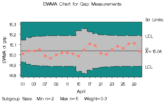
The following statements request an EWMA chart, shown in Output 20.3.2, for these gap measurements:

   title 'EWMA Chart for Gap Measurements';
   symbol v=dot c=salmon;
   proc macontrol data=clips4;
      ewmachart gap*dayc / weight   = 0.3
                           cframe   = vibg
                           cinfill  = ligr
                           coutfill = yellow
                           cconnect = salmon;
   run;

The character variable DAYC (rather than the numeric variable DAY) is specified as the subgroup-variable in the preceding EWMACHART statement. If DAY were the subgroup-variable, each day during April would appear on the horizontal axis, including the weekend days of April 5 and April 6 for which no measurements were taken. To avoid this problem, the subgroup-variable DAYC is created from DAY using the PUT and SUBSTR function. Since DAYC is a character subgroup-variable, a discrete axis is used for the horizontal axis, and as a result, April 5 and April 6 do not appear on the horizontal axis in Output 20.3.2. A LABEL statement is used to specify the label April for the horizontal axis, indicating the month that these measurements were taken.

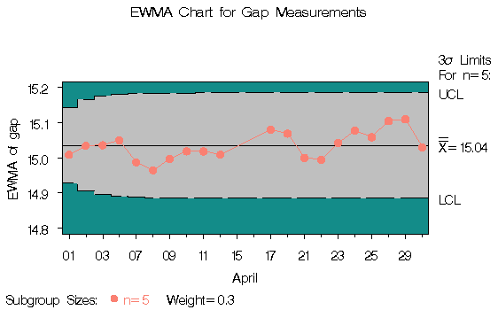
The EWMACHART statement provides various options for working with unequal subgroup sample sizes. For example, you can use the LIMITN= option to specify a fixed (nominal) sample size for computing control limits, as illustrated by the following statements:

   proc macontrol data=clips4;
      ewmachart gap*dayc / weight   = 0.3
                           limitn   = 5
                           cframe   = vibg
                           cinfill  = ligr
                           coutfill = yellow
                           cconnect = salmon;
   run;

The resulting chart is shown in Output 20.3.3.

   proc macontrol data=clips4;
      ewmachart gap*dayc/ weight   = 0.3
                          limitn   = 5
                          alln
                          nmarkers
                          cframe   = vibg
                          cinfill  = ligr
                          coutfill = yellow
                          cconnect = salmon;
   run;

The chart is shown in Output 20.3.4. The NMARKERS option requests special symbols to identify points for which the subgroup sample size differs from the nominal sample size.

The following statements apply all three methods:

   proc macontrol data=clips4;
      ewmachart gap*dayc / outlimits = cliplim1
                           outindex  = 'Default'
                           weight    = 0.3
                           nochart;
      ewmachart gap*dayc / smethod   = mvlue
                           outlimits = cliplim2
                           outindex  = 'MVLUE'
                           weight    = 0.3
                           nochart;
      ewmachart gap*dayc / smethod   = rmsdf
                           outlimits = cliplim3
                           outindex  = 'RMSDF'
                           weight    = 0.3
                           nochart;
   run;

   title 'Estimating the Process Standard Deviation';
   data climits;
      set cliplim1 cliplim2 cliplim3;
   run;

The data set CLIMITS is listed in Output 20.3.5.

Chapter Contents

Previous

Next

Top

Copyright © 1999 by SAS Institute Inc., Cary, NC, USA. All rights reserved.