In
the previous module, we have summarized the behavioural aspects
of sound propagation in open and enclosed spaces, with some
references to the psychoacoustics involved. Here we will extend
our enquiry into one of the most important topics in soundscape
studies, namely the perception of acoustic space.
We will begin with auditory localization via binaural hearing,
and the related topic of binaural recording, and then progress
to the ways in which the sense of acoustic space is created
by sound, and how it can be documented.
home A. Binaural Hearing. Our ability to
hear spatially is termed binaural
hearing because it is normally done with both
ears. The two auditory nerves, one for each ear, join part
way up the path to the brain at which point the two sets of
electrical impulses can be compared and interaural
differences can be detected.
The auditory system’s ability to detect direction is called
localization, and is the most accurate in the
horizontal plane (left to right) where the angle of a source
compared with the frontal direction is termed the azimuth,
following its use in astronomy for the angle of, for
instance, a star’s location compared with north. As such, it
is measured in degrees, with 0° in front, 90° on the
righthand side, 180° at the rear, and 270° to the lefthand
side. Similarly, elevation can refer to the
perceived height of the source.
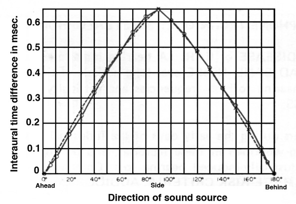
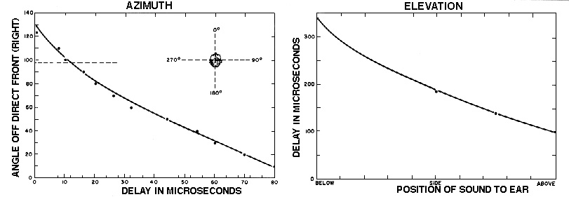
The two most basic variables for
localization are the interaural time differences
between the ears (ITD) and the interaural
amplitude differences (IAD), or interaural
intensity differences (IID). The time differences are caused
by the different distances the sound travels to each ear,
starting with zero difference as shown below for direct
front and direct back in terms of source location, with the
differences increasing to about 0.65 ms at the right
(90°) and left (270°). Given that the size of the head is
less than 1 ft (.3 m), this delay range is quite predictable
as shown in the diagram at the left.
Click to enlarge either image
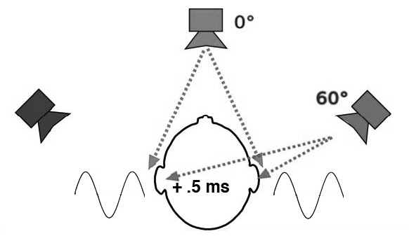
That is, the
ITD assumes that the wave is able to diffract
around the head, which as we documented in the previous module,
only happens for low frequencies with long wavelengths. In the
righthand diagram, the low frequency source at 60° will diffract
around the head and arrive at the far ear with the same
amplitude, but about .5 ms later. In general, then, we can only
localize low frequencies below about 1500 Hz via
interaural time delays.
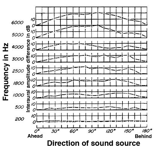
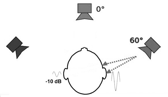
Above that range, higher frequencies cannot diffract
around the head, thereby creating a sound shadow on the
opposite side. This means there are significant IAD’s
(interaural amplitude differences), and as shown here, they can
be as high as 20 dB for the far right and far left directions
(as shown for 5 and 6 kHz). A 4 kHz source at 60°, for instance, will
arrive at the far ear with a 10 dB attenuation.
Click to enlarge either image
12. Personal listening
experiment. Find an environment with a fairly
steady high frequency component in the soundscape, e.g. a hiss
or broadband sound from a motor or fan, or perhaps a light
that is buzzing. Move your head around and you will easily
hear the high frequencies getting louder and quieter in each
ear. Note that something similar will not and cannot happen
for low frequencies.
High
frequency hum in a mechanical room at UBC
Source: WSP 19 take 5
You can try the same experiment with this recording played on
speakers. Listen to this broadband sound while moving your
head around. The nasty high frequency hum around 3 kHz (where
the ear is most sensitive) will change in loudness as you
move, but not the lower part of the drone.
So, we can
summarize the effects below and above 1500 Hz:
low frequencies are localized by ITD
(interaural time differences) high
frequencies are localized by IAD (interaural amplitude
differences)
Keep
in mind that the spectrum of many sounds has energy in both
regions, so that doubles up, so to speak, on our ability to
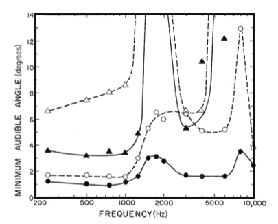
localize them. However, the following diagram shows the jnd for
direction, known as the Minimum
Audible Angle, that is, the smallest change in
direction one can hear. The curves go from the bottom at an
azimuth of 0° (black circles), through 30° (white circles), 60°
(black triangles), and 75° (white triangles) as the highest.
Minimum audible angle for various
frequencies and directions
It is clear
that the jnd is lowest (around 1° accuracy) for straight
ahead (an azimuth of 0°), which correlates with the direction of
the eyes. Therefore, it is not surprising that we turn to face
the direction of a sound we want to localize where we have both
the best visual and aural acuity. Also, note that our ability to
localize drops off quite sharply as the angle of the source
moves towards the side of the head. And our acuity around 1500
Hz is poor, but few sounds are specifically placed in that
frequency range.
Here are some demo's of ITD's that you can (only) hear on
headphones.
Localization with only ITD, interaural
time differences. Source: IPO73
The same effect in smaller steps with
percussive sounds
Switching interaural phase differences
of 45° for 500 Hz and 2 kHz tones. Source: IPO72
The last example refers to a phase difference,
but keep in mind that a phase difference is simply a very
small time difference, on the order of magnitude of a
fraction of the period of the wave. For the lower frequency (500
Hz) you can hear a spatial shift with these phase switches, but
for 2 kHz you cannot. This is because at high frequencies, a
phase shift is very small and not unique, in the sense that it
could be 1/2 wavelength, or 3/2 or anything similar, and
besides, these tones would not diffract around the head. Front and Back. You may have
already noticed an implied symmetry between front and
back in terms of the ITD and IAD that we experience with two
ears. For instance, a source either at the front or back arrives
at the ears simultaneously, and likewise sound coming from the
back has the same issue of diffracting around the head or not.
The other omission in this model is the lack of reference for
elevation, or height. That is because the models have assumed a
more or less spherical head shape. Obviously the eyes favour the
front of the head, but so do the ears – that is, the outer ear
flaps, the pinna (plural: pinnae) face forwards as well.
The ridges of the pinna play an important role in localization
for front and back distinctions, as well as higher and
lower elevations. This is because the sound wave bounces off
those ridges with very small time delays (in the microsecond
range, compared with the millisecond range for the ITD), and
then combines with the direct sound resulting in the
cancellation of certain frequencies.
In the last module, as
well as in an electroacoustic module,
we showed that such small time delays in phasing cause a
comb filter effect with out of phase frequencies
cancelling, specifically the odd harmonics. The “colouring” of
the high frequencies occurs around and above 8 kHz.
The first pair of diagrams below shows the kind of time delays
(up to 80 microseconds) involved in bounces off the inner ridge
(left) which give a colouration to frontal sounds and not to
those from the rear. The longer delays (several hundred
microseconds) off the outer ridge (right) change the colouration
for higher elevations. Each of these causes a notch in the
spectrum.
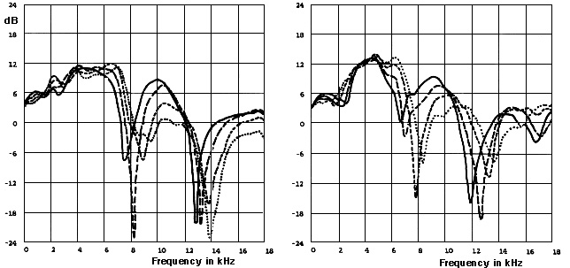
The second pair of diagrams shows the Head-Related Transfer
Function (HRTF) for two different ears, which means the
spectrum filtering caused by these delays, with the typical
notches around 8 and 13 kHz.
Head-related
transfer functions (HRTF) for two subjects. Solid
lines are for 0° elevation, long dashes for 10°, short
dashes for 20° and dotted lines for 30° elevation.
Note the small differences between subjects, while
retaining the same basic comb filter shape. (Source:
Kendall & Martens)
We will refer to this effect as pinna
colouration, and obviously it is a subtle phenomenon. Keep
in mind that hearing loss with age (presbycusis)
can attenuate hearing sensitivity in this high frequency range.
We obviously become used to our own specific version of this
colouration, although tests with averaged values have shown that
the notch cues are sufficiently strong to be interpreted from
those values. We will discuss below the issues involved in
recording these cues with binaural recording systems. Front-back
“flips” in perceived direction are commonplace in many
situations.
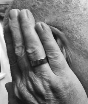
13.
Personal listening experiment. Work
with a friend, preferably in a relatively open space
where you’re not getting reflections off nearby
objects. Practice holding your hands over your ears
such that the pinnae are covered but not the
entry way to the ear canal while keeping your hands
upright,
ideally a bit moreso than in the photo.
Have your friend snap fingers (or activate a clicker)
in front and behind you at about a distance of two
feet, right in the centre each time while you guess
“front or back”. If you mistake a front click for a
back one, have your friend tell you to open your eyes.
The auditory system is very good at “learning” this
kind of situation by finding other clues to the
problem, so try to do the experiment quickly and with
minimum movement on the part of your friend. Once you
get a sense of your degree of accuracy with the pinna
blocked, go back to no blockage and try the experiment
again – probably with much better accuracy.
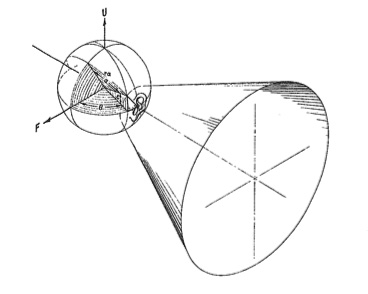
Finally,
just as localization acuity is best in the front, it is quite
poor at the sides of the head over a three-dimensional area
colourfully called the Cone of Confusion (perhaps moreso
some days than others). As in this diagram, every point on the
surface of the imaginary cone at the side of the head can be
confused with any other due to the symmetry involved. This can
also be tested similarly to the above experiment but not with
the pinna blocked.
B. Binaural Recording. Standard
microphone recording formats do not include the binaural cues
that we have documented in the previous section. The
interaural time differences (ITD) will not be present unless
the microphones are placed at a similar distance that the ears
are apart. The interaural amplitude differences (IAD) for high
frequencies will also be absent since microphones are smaller
than the size of the head, and any lack of diffraction around
the microphone will be at even higher frequencies. And, of
course, pinna colouration will be completely absent. Finally,
any effects from the head and torso will also be missing.
Listening to a typical recording, particularly one done in a
sound studio, will produce in-head localization (IHL).
That is, the apparent location of the sound will be inside
your head. This effect can arise when there are only amplitude
differences between the left and right channels, a process
called panning
the signal.
The brain is unused to having two sounds arrive at the ears
differing only in amplitude, and so the perception is not “two
sounds” from “two locations”, but “one sound” from an
“averaged location”. When the amplitudes are exactly the same,
that location will be in the middle, and the perceived image
is suggestively called a phantom image.
In the next module, we will show that with loudspeakers, the
phantom image is highly unstable, and if you move
slightly to the left or right of the exact middle between the
speakers, the image will collapse to the nearer speaker, as a
result of precedence
effect. However, when your head is in a fixed
location relative to the speakers (as is the case with
headphones), the “exact middle” is inside your head.
Prior to stereo audio, hearing “voices and music inside your
head” might qualify you as prone to hallucinations,
schizophrenia or worse, but after a century of it being
“normal”, or at least customary, a reversion to what the
unaided ear experiences – sounds being localized exterior
to the body – is often surprisingly surprising! But that
is what some experimental recordists and audio engineers
started experimenting with since the 1930s.
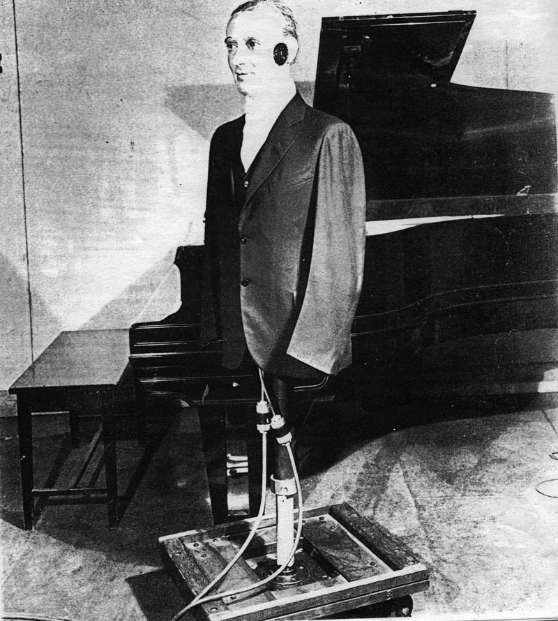
Possibly the first example was a mannequin named “Oscar” at
Bell Labs which had microphones in the place of ears, but only
rudimentary pinnae. Then as now it was tempting to have
someone listening via headphones while sounds were made in
close proximity to the microphones, just to see how they’d
react. However, there was no medium for stereo recording or
broadcast at that time, so the experiments didn't lead
anywhere.
The mannequin known as Oscar at Bell Labs, 1930s (click to
enlarge)
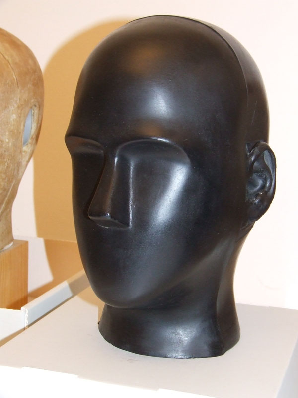
In
the 1960s, the Neumann microphone company in Germany
experimented with what they called a kunstkopf, or "artificial
head” (popularly know as a “dummy head” with all of the
expected humour attached). It modelled the pinnae fairly
accurately, and the microphones were placed at the location of
the eardrums inside the ear canal. The listener needed to hear
the recording on headphones (not speakers) so that there was no
second layer of pinna colouration (by passing over the
listener’s pinnae again).
Kunstkopf
recording at a German beer garden in Munich, 1970s
(ordering a cola) with a Neumann kunstkopf
(at right)
Neumann researchers experimented with adding a torso which
contributed some nuances to the realism, but experiments with
adding hair were a predictable failure. The main problem with
binaural recording seems to be to get a well-defined
frontal image where the pinna colourations need to be
precise. Of course, if a trajectory path is suggested, then
the listener will likely hear it passing in front, with
possibly a slight rise in the middle. Going over the head is
also a tricky image to sustain, as in this example, first left
to right (quite good) then from centre to above the head (a
bit more problematic).
Left
to right trajectory around an artificial head, then front
centre to above the head. Source: Cook 26
Some of
the best binaural recordings are those made by Richard Duda
at San Jose State University in California, in his lab
equipped with a Kemar artificial head. The Kemar includes a
modelled torso, and accurate pinnae.
Kemar
in an anechoic chamber; back view of microphones
Moving
from a reverberant room to an anechoic chamber
Binaural
cues in the frontal plane (left, above, right,
below)
Music
in 3 examples: Left track mono; Right track mono;
binaural
Check out the clarinet over your right shoulder!
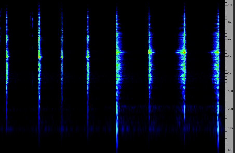
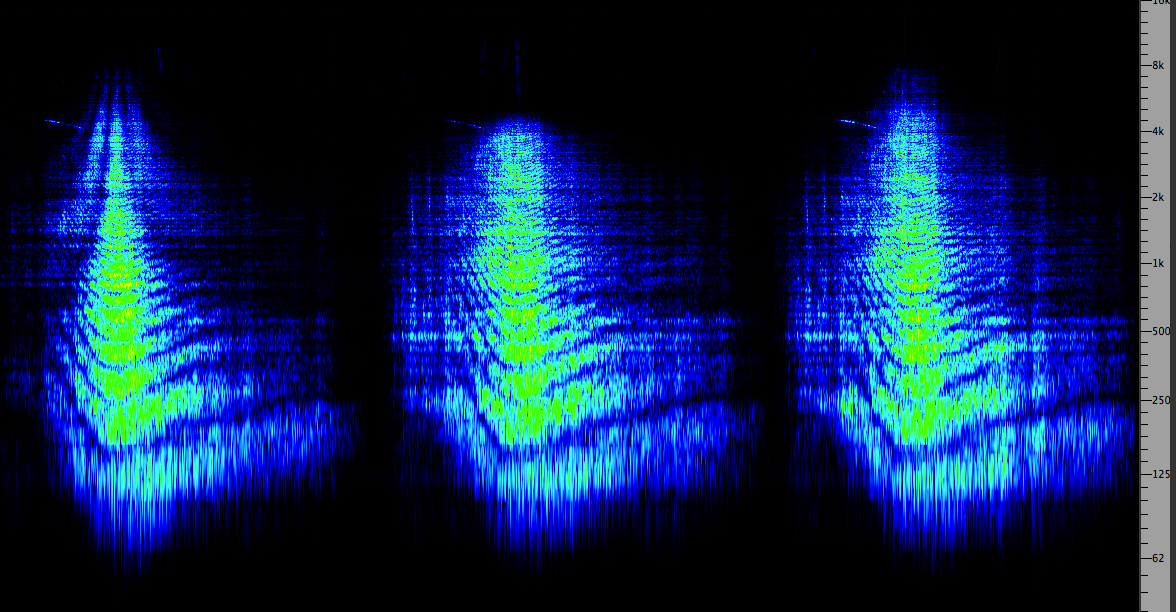
Passing jet in 3 examples: Normal
stereo; Low-bandwidth binaural; High-bandwidth
binaural; Spectrogram
Which gives the best impression of the jet being
overhead?
Source: Duda
Once we have HRTF data, it is possible to
simulate 3-dimensional localization and movement with purely
digital processing. Here are two examples created by Gary
Kendall.
Chainsaw
The original chainsaw, heard first, was recorded in a
stationary position, then using HRTF processing it
appears to fly around you (try not to duck!)
Footsteps
The footsteps are recorded moving in place, and then
processed as if they were first in a dry, then a
reverberant stairwell. Do the steps go up or down?
Does your contextual knowledge of stairwells help the
vertical localization?
Today,
binaural microphones often are designed to be worn in the
recordist’s ears, which of course is less obtrusive and more
portable (see the Field Recording
module). However, it raises the issue of head movement
on the part of the recordist, and how it will be interpreted by
a listener whose head is presumably stationary. Also, there will
likely be differences between listeners as to the degree to
which the sound image is localized outside the head, given the
tradition of headphone listening producing in-head localization.
Here are two final examples, the first of a fireworks recording
using an artificial head, and the second, a famous and very
entertaining binaural drama, the Virtual Haircut.
Fireworks
display in Vancouver. Source: WSP VFile 2, take 11
C. Psychoacoustics of localization. In
the sections above, we have identified the basic acoustic
localization cues of time and amplitude differences between the
ears, and spectral colouration in the high frequencies created
by the outer ears, the pinnae. Together they form the basic
sources of information used in binaural hearing, and in
the previous section we have given examples of how such cues may
be captured in binaural recordings.
Here we will present two “effects” that take place in the brain
that play a role in sorting out these cues in order to create a
sense of acoustic space. They are called the cocktail party
effect and the precedence effect, and together
with other cues, they assist in what is generally known as auditory
scene analysis. This refers to the study of how two
binaural inputs to the brain result in an image of specific
sources within an overall “scene”, in this case, a soundscape.
Both effects are based on the brain’s ability to inhibit
certain input signals (i.e. neural patterns) while enhancing
others. When we do this consciously, we say we are focusing
on a particular sound, however, with precedence effect, the
inhibition of late arriving signals is done automatically.
Cocktail party effect, as it is rather
colourfully called, refers to our ability to identify and focus
on a specific source in the midst of other sources. The implied
example is of a crowded social space where many voices are
simultaneously speaking, and our ability to focus on one or two
of them. First we need to identify what sounds “belong” to each
speech stream, and the most important cue to do that is the
direction and location where they come from. Sounds coming from
the same direction and location (i.e. distance) are
assumed to be from the same source.
These two examples begin by removing the spatial cues, and then
restoring them. The first is in conventional stereo where the
left and right channels are mixed together (but with the same
voice, just to make the task a bit harder), and then separated
into left-right stereo. The second uses a binaural recording
doing something similar by playing the two short texts
separately, then combined. These examples work on both
loudspeakers and headphones.
Same
voice with mixed texts, mono then stereo
Two
texts, one at a time, then mixed; source: Duda
14. Personal
listening experiment. The next time you are in
a relatively noisy public space where there are many voices,
try focusing on individual ones without looking at the person
speaking. You can also close your eyes. Besides some that are
clearly louder, are there others that are easy to follow? Can
you tell why that is the case? If there are other languages
being spoken, does that make it harder?
Now, try
the same experiment at a party or other situation where you
know many of the people speaking. This will probably be easier
to do. Can you simultaneously carry on a conversation with
someone beside you while doing this? Some people find this a
useful social skill that may have helped with the naming of
the effect!
The above
examples probably brought out several variables such as your
prior familiarity with a particular voice and of course the
language being used. The relative superficiality of the
conversations you heard, the familiar clichés as well as the
lack of complex prose structures, all combined to make the
perceptual task easier.
However, it also turns out that some people simply have more
“distinctive” voices that are more easily recognizable, and not
just because of loudness. It probably has to do with a specific
timbre, or perhaps the typical paralanguage they
use (as discussed in the Speech
Acoustics module). And finally, in the case of the party
with people you know, you may have noticed your own motivation
to being drawn to a specific voice when you have a personal
stake in the conversation, or relationship with the person
involved. Nothing like hearing someone say your name to get your
attention – even if it turns out they are referring to someone
else!
There is also a darker side to this listening
phenomenon – it is one of the first to be impaired with hearing
loss, as discussed in the Audiology
module. As we will demonstrate there, hearing loss, particularly
in the critical speech frequencies, involves a broadening of the
spectral resolution along the length of the basilar membrane, in
addition to a loss of overall sensitivity. In other words, the
problem is not the lack of loudness, but the lack of clarity
and definition in hearing.
Therefore, those with impaired hearing instinctively avoid
crowded environments or those that are noisy enough to make
discerning speech very difficult, which can lead to
self-isolation and reduced interpersonal interaction. The
ability to separate a voice from background noise, or other
simultaneous voices, as you have done here under idealized
acoustic conditions, becomes impaired.
Precedence effect. For those with
unimpaired hearing, the main psychoacoustic cue that lets the
auditory system separate the direct sound from the reverberated
sound, is an ability called precedence
effect (or the Haas effect, after its discoverer
Helmut Haas), as described in the previous module, but worth
repeating here:
-
the direct sound arrives first as a coherent (i.e. correlated)
sound wave since all frequencies travel at the same speed,
even if they are coloured along the way, and is
likely to be stronger than the reverberant sound
- the
reflected sound arrives later and is uncorrelated
because of the random nature of reflections with their
various time delays
The effect itself is the auditory system’s ability to inhibit
the neural impulses that arrive up to 40 ms after the
original sound, in an attempt to minimize their ability to mask the original
sound. In other words, the effects of reverberation are
regulated, even though we remain aware of its effects on the
sound. However, excessive reverberation will still likely
overpower the effect and result in reduced comprehension.
Personal haptic
experiment. Precedence effect can be
experienced in other forms of sensory input, not just sound.
Try this experiment.
1) Tap your two index fingers together. Do you feel equal
pressure on both fingers as the site of the stimulation?
2) Tap your
index finger on your lips. Which is the site of the stimulus –
lips or finger?
3) Now tap
your ankle with your index finger. Which is the stimulus site
now? Answer here.
The effect is
so named because the auditory system gives “precedence”
to first arriving signals, and suppresses later arriving
ones. In acoustic situations, the first arriving sound, the
direct signal, is always louder, as reflections will have lost
some energy. However, in electroacoustic situations where
amplification is involved, the signal sent to a nearby
loudspeaker will arrive before the acoustic one, and
will likely be louder, so the loudspeaker is the apparent
source.
Listeners often don’t realize this if they can see the original
sound source, such as a performer – until they close their eyes,
and maybe then they will recognize the actual direction from
which the sound emanates. Some spaces are equipped with built-in
delays for amplified sound to avoid this situation.
Situations where a reproduced sound is louder but not first
will be confusing. If the delay to the later, louder sound isn’t
too long, it will likely override the acoustic version, but if
it’s longer, it will likely be heard as a separate, echoic
event. In a very large outdoor stadium with an amplification
system, there is likely to be a lot of aural confusion as
delayed versions collide with the nearer loudspeakers. It’s a
good listening experiment in any situation involving
acoustic and amplified sources to analyze what is actually going
on and why.
The traditional demonstration of the precedence effect is to
listen to sounds in their forward and reversed
directions and compare the aural impression of how long the
reverberation lasts. In the first example, we hear a brick
struck twice in a low reverb space, followed by its reversal,
and then in an reverberant space, followed by its reversal. Does
the length of the reverb sound longer when it is heard first?
And if so, by approximately how much? Answers here.
Brick
struck twice in low and high reverb situation, then
reversed
Click
to enlarge
Reversed
speech in reverberant space played backwards so the
reverb occurs first (Source: Christopher Gaze)
In the second example, we reverse speech in a reverberant space,
and then play the result backwards, so that the reverb portion
now precedes the original. The direct sound, being
louder, overwhelms the reverb version, but the reverberant
portion is almost decorrelated enough to sound like a separate
source which of course cannot happen in the normal forwards
version.
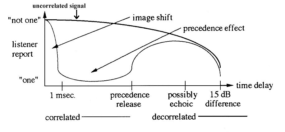
In the above
diagram, Gary Kendall summarizes listeners’ subjective
impressions of correlated and uncorrelated sound sources
based on the delay time of arrival. For very short delays, less
than 1 ms, we get the binaural shift similar to the interaural
time difference referenced above for a position moving away from
direct centre to the side (called “image shift” in the diagram).
Above that, the precedence effect kicks in for about 40 ms. If
the signal is correlated (the lighter bottom
line), this quickly reinforces a singular image (marked “one”).
With the release of the precedence effect, the image is
“possibly echoic”.
However, if the delayed signal is uncorrelated (as with
our reversed reverb example above), or is decorrelated by signal
processing (the darker upper line), it starts behaving
like any other uncorrelated sound in the environment. For
instance, separate sources are by definition uncorrelated, so in
the cocktail party effect, you could focus on individual voices,
particularly when they came from different directions. In this
diagram, the uncorrelated sounds maintain their “not one” image
for all time delays.
Kendall’s interest in this problem stemmed from
multi-channel electroacoustic sound diffusion with
multiple speakers. The studio practice of panning sound
between channels, as referred to in section A,
means that only the amplitude of the sound in each
channel is varied. This keeps the signal correlated, and its
apparent location is called a phantom image. However,
once the listener is even slightly closer to one speaker, the
source of the image collapses to the nearer speaker
because of precedence effect (since the sound from the farther
speaker is weaker and arrives later, and hence its presence is
inhibited).
15. Personal Listening
Experiment. In fact, go back to the first example under cocktail party effect
(the female voice in a mix of two statements) and listen to it
on speakers that are at least 6’ (2 m) apart. Start by trying
to be exactly in the middle between the speakers and hear
whether the image is localized there as well. Then move 1 foot
(several centimetres) to the right or left, and notice how the
image will collapse to the nearer speaker.
In Kendall’s
case, he was interested in keeping delayed signals uncorrelated
so they would be heard separately (the “not one” image). In
fact, what he was doing was replicating the normal situation in
a soundscape where almost all sources are uncorrelated, which
allows us to hear them separately. Just like binaural recording,
this is a return to what we might call the “acoustic normal”,
as distinct from the electroacoustic “normalization of the
artificial”. As such, uncorrelated sound sources are the
basis of the perception of acoustic space.
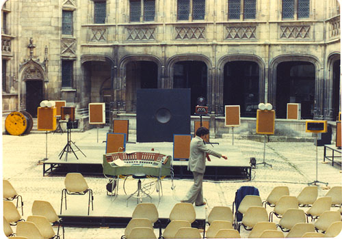
An early electroacoustic sound diffusion setup in the Palais
Jacques Coeur, in Bourges, France, in the 1970s.
A centrally placed mixer allows the composer/performer to
route a stereo signal to any speaker present in varying
amounts. Speakers were deliberately mismatched so they would
contribute their own colour, but still work in stereo pairs.
On the other hand, stereo electroacoustic
diffusion, that is, the performance of a stereo soundtrack
through multiple speakers placed around a space, has always
depended on the positive aspect of the precedence effect.
Using a mixing board placed in the middle of a hall, the person
diffusing the stereo work can raise the level being sent to a
particular speaker, and even if the sound is also going to all
others speakers, at a lower level of course, the sound will
appear to come from the speaker where the enhanced signal is
placed.
Then, by rapidly alternating speaker levels at different
locations and heights, usually in synch with particular sounds
on the track, there is a very convincing aural illusion that the
sound is not just stereo, but an immersive 3-dimensional
soundscape with moving source sources. The main limitation is
that only one sound at a time can be moved around in this
manner.
D. Acoustic Mapping. Before we summarize
all of the aspects that are involved in the aural creation of
acoustic space, let us add some spatial concepts contributed
by the World Soundscape Project (WSP): the acoustic
profile and the acoustic horizon.
The acoustic
profile is a map of how far any given sound
source can be heard, or in the case of a community, how
various profiles overlap and interact. In the WSP’s first
study, that of Vancouver in 1973, an acoustic profile map was
created for the Holy Rosary Cathedral bells in the downtown
core. The profile for this set of bells (of the type used for
English change ringing), was just a few blocks in the early
1970s, as shown below, despite aural history accounts from
locals that they were able to be heard several miles away in
south Vancouver earlier in the century.
Acoustic
profile of the Holy Rosary Bells, Vancouver, 1973 (source: Vancouver
Soundscape)
What had happened in the interim was twofold: the increasing
ambient noise level of the city, particularly in the downtown
core, and the construction of much higher buildings around the
church. Archival photos of the church from 1920 show that at the
time it was the tallest building in the area, so residents even
far away had direct “line of sight" to its towers.
Recently in 2015, a group of students repeated the exercise, and
discovered that the profile had shrunk again, particularly in
the southerly direction (at the left) where the bells could not
be heard past Georgia or Robson streets. The basic acoustic
function of the profile is to allow everyone located within its
radius to potentially have the shared experience of
hearing the sound source. In historic periods for church bells,
it marked the extent of the parish. Now, in more secular
times, it is traffic and aircraft that can be heard throughout
the community.
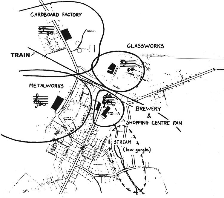
Acoustic
profiles in Skruv, Sweden (click to enlarge)
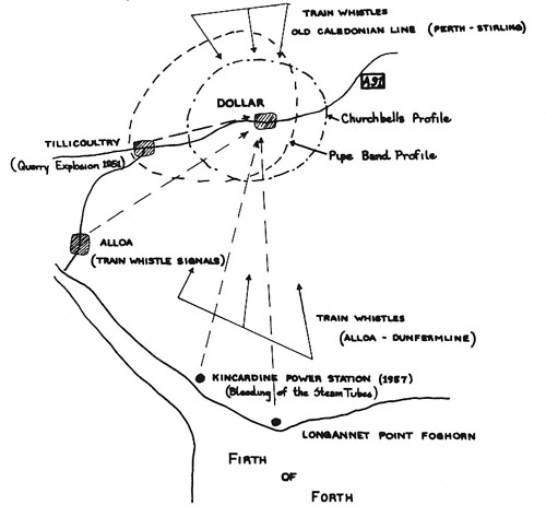
Two acoustic profiles in Dollar, Scotland, the pipe
band and the churchbell
This
diagram at left shows the minimal overlapping of factory hums
in a relatively modern industrial village in Sweden (Skruv).
The village is bisected by a train line, and there’s a
partially submerged stream as well in terms of permanent
features of the soundscape. At the right are the two profiles
for specific soundmarks in a Scottish village
(Dollar), the pipe band and the church bell, showing how they
span the entire village and beyond. Both villages were part of
the WSP’s Five Villages study.
Compare these acoustic profile maps to the isobel map
which documents sound level contours that join points of equal
level measurements, as shown here.
Acoustic horizon. From the reverse
perspective of incoming sounds, as opposed to
outgoing ones from a local source, the acoustic
horizon can be defined as the most distant
sounds one can hear at any position. Clearly, both the
profiles, and in particular, the acoustic horizon, will vary
according to time of day and local atmospheric conditions as
presented in section A
of the Sound-Environment Interaction module.
The acoustic horizon of two communities: Bissingen, Germany
(left) and Lesconil, France (right)
At the left is a map of the region around Bissingen, Germany,
that refers to which bells from neighbouring villages could be
heard in Bissingen in the past, based on interviews with older
residents. At the right is a diagram that documents how the
acoustic horizon shifted during the day at Lesconil, France, a
fishing village. The daily wind pattern (les vents solaires)
for offshore winds in the morning and onshore winds in the
afternoon, correlated with the traditional fishing boat
schedules at a time when the boats were dependent on wind
power.
The shifting winds also meant that particular foghorns and
other sounds could be heard in the village at specific times
of day. The diagram also represented a norm that could be
deviated from with more unsettled conditions. These historical
observations, gleaned from interviews, are useful in
documenting how the acoustic community changes over time.
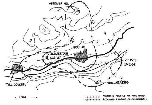
Two acoustic profiles of Dollar, Scotland (pipe band and
churchbells), plus incoming sounds from other locations
Lastly, the
acoustic profiles in Dollar, shown above, are compared with
distant sounds on the acoustic horizon of the village. In
particular, two railway lines, one to the north and one to the
south could be heard in the village, as well as two sound
sources near the Firth of Forth, a power station and a
foghorn, all of which are indicative of the geographical
context of the community.
All of the examples in this section are
reminders of how acoustic space changes over time and how
acoustic knowledge about its character contributes to a sense
of place and community. Since change is inevitable, on
both the short-term and long-term scale, questions will arise
as to whether the system as a whole can adapt or will
something be lost. The loss of any specific sound (a disappearing
sound) may result in a form of nostalgia for
residents, and may even create the impression of a sound
romance that symbolizes a past relationship.
However, the more important question may be whether the
soundscape as a whole is sustainable, by which we
mean, our ability as a culture to live within a positively
functioning soundscape that has long-term viability.
E. Acoustic Space. In all five of the
acoustic modules thus far, we have been laying a groundwork
for understanding a key concept for understanding
soundscapes as an eco-system, namely what we are calling acoustic
space. Speech and music have their role to play as
specialized forms of soundmaking, but acoustically they work
within the same contexts of acoustic space and interact with
them. Although we still have some important concepts to deal
with in the next module, Sound-Sound Interaction, including
how the auditory system separates simultaneous sounds, this
is probably a good point to summarize the main points about
acoustic space. We will also add some links to relevant
material in the Tutorial, not the Handbook in
this case.
- the perception of acoustic space is created by
sounds and sound events, and therefore is entirely dependent
on time (that is, it is the result of movement), whereas
visual space produces a largely stable sense of space that
can include movement; physical space is the objective space
we can move through and measure
- acoustic
spaces, while multi-dimensional, can be placed along a
general continuum
where interactive spaces are in the middle, with the
extremes of the continuum being anechoic conditions and
diffuse sound fields
- at the
micro-level of the interaction of sound waves arriving at
the ear, binaural cues allow the auditory
system to localize the direction and distance of sounds
- the
auditory system effortlessly decodes two types of information in the arriving sound, the
character of the sound source as activated by some causal
energy (through the coherent vibration that arrives first)
and the character of the physical environment within and
through which the sound has travelled (through the random
uncorrelated reflections that arrive later)
- sounds
that arrive from the same direction (or continuous range of
directions) with a similar timbre and temporal behaviour are
deemed to be from the same source, and
under favourable conditions, can be distinguished from other
sources
At
this point, we have outlined or at least referred to, all of
the factors that we know are involved in creating what Albert
Bregman calls an “auditory scene”. Let’s listen to an
example that shows a certain degree of complexity as to how it
works.
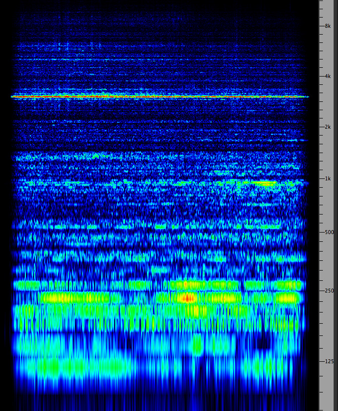
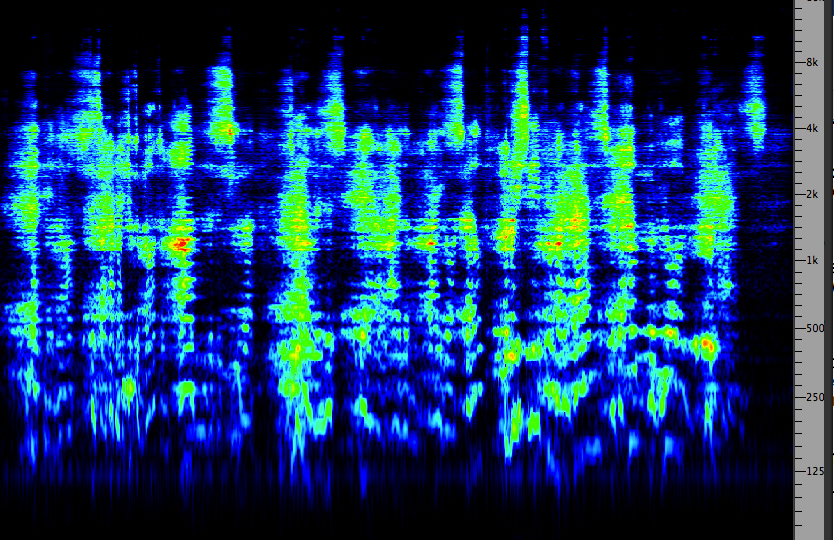
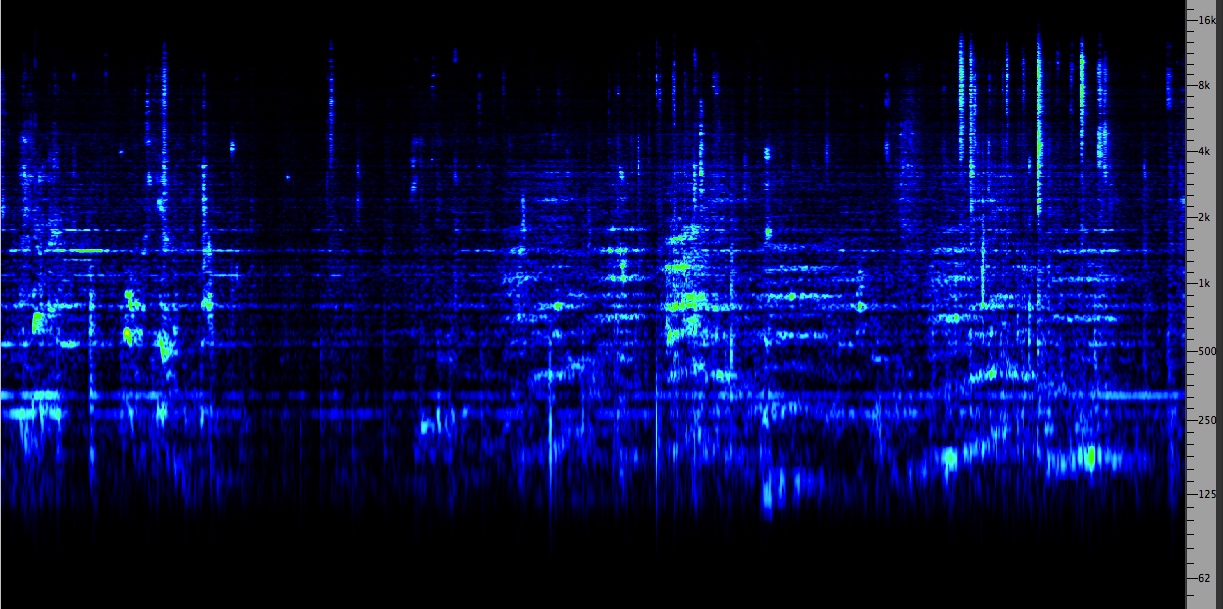
This recording was made in Cembra, Italy, by the WSP during
its Five Villages study. There are three components to
the acoustic space: (1) foreground sounds of men chatting and
moving on the cobblestone pavement (2) a distant sound of
church bells that marks the periphery or acoustic horizon of
the soundscape (3) a choir from a different church in the
middle ground, heard coming from the inside.
Notice how effortlessly this auditory scene is established and
with what degree of clarity or definition. Note that the
spectrogram, while useful, does not clearly separate the three
levels of spatialized elements.
Cembra,
Italy, auditory scene
(Source: WSP Eur 33 take 1)
Click
to enlarge
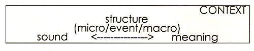
The next stage becomes communicational
as we consider the types of information that have been
communicated through this type of perception of acoustic
space.
- our ability to recognize patterns
within the sound yields information about the event
itself, such as its identification and causality, and our
knowledge of context allows us to interpret the
meaning that can be ascribed to that information
- aided
by other sensory input, the perception of acoustic space
gives us a primary sense of orientation within any
given space, or sometimes its opposite, disorientation
where we need to rely on other types of information
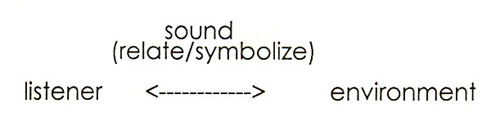
-
relationships to other people, social groups and
political/economic entities, and to the community as a
whole are established and reinforced by repetitive
acoustic experience
-
repeated and ubiquitous relationships that have been mediated
by sound can come to be symbolized by the sound
itself, at both the individual and community level
Although
many details remain to be filled in, this model attempts
to summarize how specific aspects of acoustics,
psychoacoustics and communication come together to form a
general model of an acoustic eco-system. Once that becomes
clear, we can consider how the impact of electroacoustic
technology, as well as noise, impacts such a system.
For instance, do such changes degrade or enhance the
system? How can design practices improve unstable and
malfunctioning soundscapes? Can alternatives be imagined
and implemented? These are much larger questions, probably
beyond the scope of this document, but clearly (I
maintain) their answers will depend on a solid knowledge
about sound as documented here.

Note: All sound examples in topics A and B need to be listened to with high quality headphones or earbuds.

