|
MAGNITUDE |
Intensity and Loudness
|
MAGNITUDE |
Most analytical categories for sound treat it in the two dimensions of magnitude (which might be thought of as a "vertical" dimension) and time (the corresponding "horizontal" dimension that we have documented under Vibration). The term magnitude can apply both to the scientist's desire to measure and quantify the physical size and energy of the sound wave, and also to the listener's subjective evaluation of the loudness and/or volume of the aural experience. The following sections present the concepts of magnitude in six sub-topics:A) The physical parameters used by the acoustician to describe the magnitude of the sound wave
B) The various "level" measurement systems which quantify magnitude on a logarithmic scale
C) The description and measurement of the subjective sense of loudness
D) An alternative concept: volume
E) Temporal aspects of loudness
F) The envelope of a sound, how its magnitude changes over time
P) Downloadable pdf summary of Magnitude (control click or right click to download)
Q) Review Quiz
The level measurement systems introduced in B) naturally lead into noise measurement systems, almost all of which are principally concerned with measuring the magnitude of noise, and community response to it. Given the specialized nature of this topic, it is dealt with separately in another module.
home
A) The physical parameters of magnitude: the acoustician commonly uses four terms to describe the magnitude of a sound wave, each of which can be translated into an equivalent version of the other. Amplitude focusses on the size of the vibration, and sound pressure on the force which such vibration exerts on the surrounding medium. The other two terms, intensity and power, place the emphasis on the more abstract notion of the energy of the wave, thereby relating it to other forms of energy transfer and exchange.
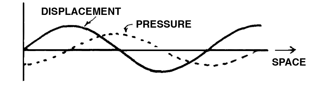
In a physical vibration, whether an acoustic wave or the movement of an object, amplitude can be used to describe either the instantaneous change of the vibration compared to its zero or “rest” position, or its maximum value. Think of a swing or pendulum, for instance, where the amplitude of its movement goes from its rest position to a maximum value, and then back again to a maximum value in the other direction. If we just say the “amplitude of the vibration”, we are usually referring to the maximum value of this change from the rest position, otherwise we should specify “instantaneous amplitude” if that is what is meant.
This diagram shows the relationship between the instantaneous displacement of a vibration and the sound pressure changes it causes. As you can see, they follow a similar pattern but are not in phase. The relationship to remember is:
maximum displacement = minimum pressure and velocity
minimum displacement (rest position) = maximum pressure and velocity
At first this might not seem obvious, but again, think of a swing. When you are at the maximum displacement of the swing, you are momentarily at rest, and therefore exert no pressure on the surrounding air. But, somewhat paradoxically, when you pass through what eventually will be the rest position, your velocity is at a maximum, and so is the pressure (e.g. wind) you experience.
When this is applied to the movement of air molecules in the atmosphere conveying sound energy, the equivalent is that the sound pressure changes are around the normal atmospheric pressure (called compressions and rarefactions). But unlike the swing, there is no “rest” position for the molecules – they are always in random motion, and so the sound wave should be thought of as a coherent pattern imposed onto this randomness.
Another, more mathematical way to think of this, is that velocity is the rate of change of position (which is mathematically the “first derivative”), and that is why it correlates with sound pressure and has a different phase than displacement.
Sound pressure itself, like all physical forms of pressure, is described in physics as force per unit area, and in air is measured in units of dynes/cm2 or Newtons/m2 or Pascals (dynes and Newtons being units of force, and the Pascal, abbreviated Pa, being a unit of pressure) or microbars (µbar) meaning in millionths of a bar where 1 bar is roughly atmospheric pressure.
Therefore, it is this pressure that activates the eardrum, setting it into analogous motion as the sound source, or activating the microphone diaphragm which reacts similarly. Therefore, we say that pressure is easy to measure, because it can be transduced by the microphone into an electrical signal, namely voltage, where it is represented as an audio signal.
On the other hand, the other types of physical parameters referred to by acousticians are energy based, namely intensity and power. Intensity refers to energy flow and is difficult to measure. It is defined as the energy transmitted per unit time through a unit area and is measured in watts/m2. Power is the total energy given out by a source in watts, and is less commonly referred to. The relationship between Intensity and Pressure is that Intensity varies as the square of the Pressure.
All such units are defined in Appendix B and given equivalents in the table in Appendix D of the Handbook.
Actually, sound represents very little in terms of energy or power, at least compared to other sources of energy we are familiar with. Every so often, someone comes up with the idea that noise pollution could be converted to an energy source, but even factory noise would hardly power a small lightbulb. If you need a break from all the physics in this section, you might enjoy the analogies that some imaginative scientists have come up with.
The energy of a 40-watt bulb falling on an area of 1 cm2 at a distance of 1 cm produces the same energy per second as 1500 bass voices singing fortissimo. [try imagining that!]
The physicist Alexander Wood once compared the human hearing range from loudest to quietest to the energy received from a 50 watt bulb situated in London, ranging from close by to that received by someone in New York.
Index
B). Level Measurements. Thus far we have been discussing the physical quantities involved with the magnitude of sound. None of the physical measurement systems, while relevant for an acoustician, are particularly appropriate for quantifying environmental sound or audio. So, what was needed is an arbitrary measurement system on a scale that is (relatively) easy to understand and applicable for everyday use. What such a system produces is called a level measurement, abbreviated capital L.
Any time the word level and the symbol L appears in a measurement, such as Sound Pressure Level (SPL) or Intensity Level (IL), these three characteristics apply:
1. Level is a measurement on an arbitrary scale, not the physical quantity itself (e.g. pressure or intensity). Therefore what we measure is a Sound Pressure Level (SPL) or an Intensity Level (IL).Formally, then, the formulas for the two most common level measurements can be expressed as:
2. A level measurement is relative, not absolute. That is, the level is always a comparison to a specific reference, such as the Threshold of Hearing.
3. A level measurement is always logarithmic and measured in Decibels (including many variations), abbreviated dB.
Intensity level: IL = 10 log10 (I / Iref) (dB)The reference intensity Iref and reference pressure pref in these equations always refer to the Threshold of Hearing which is arbitrarily assigned 0 dB.
Sound Pressure Level: SPL = 10 log (p / pref)2 = 20 log (p / pref) (dB)
In some graphs or acoustics texts, the Threshold of Hearing is identified by its formal scientific definition: 2 x 10⁻⁴ dynes/cm2 or 2 x 10⁻⁵ Pascals (Pa), which you are supposed to know is this threshold – so don’t be intimidated!
However, this is not the case with audio measurements where 0 dB refers to the maximum distortion-free level of a signal, that is, the highest level, with other audio measurements represented as negative dB, such as - 6 dB. This level is often referred to as Zero VU (where VU stands for volume unit).
The reason for this is that, first of all, there is no equivalent to the threshold of hearing in audio, just low-level background noise. Secondly, the intent with audio is to maximize the signal-to-noise ratio and avoid distortion at the top end of the dynamic scale, so everything is measured relative to the highest level, not the lowest level. If no reference is explicitly stated, then the context of acoustic sound or audio signals assumes these references. When comparing sound levels, you can also say that one sound is “10 dB greater” than another sound, thereby creating your own frame of reference.
You are not expected to know these equations – but if you’d like to take a break and let a “bedtime story” explain them to you, follow the link.
However, what is important is that you understand the implications of these level measurements, most of which derive from their logarithmic nature. The first two are:
x 2 intensity = + 3 dB
x 2 sound pressure (or amplitude) = + 6 dB
These doublings follow the fact that intensity varies as the square of the pressure (just as the scaling by 10 and 20 appeared in the IL and SPL equations above, respectively). A complete table of decibel level changes related to the Intensity Level (IL) system and to the Sound Pressure Level (SPL) system, can be found in this Handbook Appendix.
The more practical question is, do either of these doublings correspond to a doubling of loudness. The answer is not simple, as we’ll see in the Psychoacoustics section, nor is it even clear what the question means. What does a doubling of loudness really mean? Do we or can we quantify loudness as a perceptual phenomenon?
Another set of logarithmic relationships follow a “times 10” pattern:
x 10 intensity = + 10 dB
x 100 intensity = + 20 dB
x 1000 intensity = + 30 dB and so on
In these rules of thumb, the main message is that every 10 dB increase represents a tenfold change in sound intensity. So in the range of the speaking voice, roughly 60 dB, noise measurements of 70, 80, 90 and 100 represent huge leaps in energy.
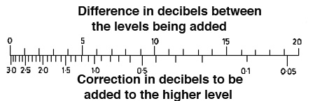
For a method of adding decibels, see the chart below under the psychoacoustic jnd for loudness based on sound pressure level differences.
Most explanations of the decibel include a table of typical examples. The choice of these is interesting in itself, but here’s one from the Handbook.
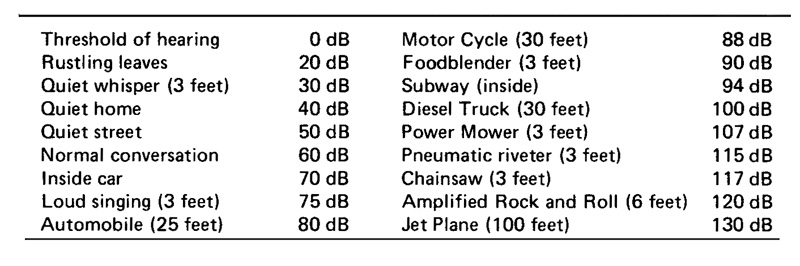
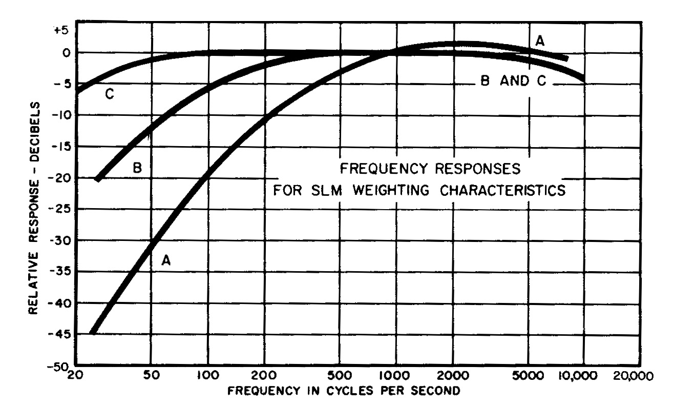
It is useful to note that in the range from 0 dB, the threshold of hearing, to 120 dB, the so-called threshold of pain (or discomfort), the human voice lies exactly in the middle around 60 dB. As humans, we have the tendency to compare ourselves, including our own sounds, to all others. What is less than 60 dB tends to be thought of as quiet, and since we can easily shout at 70 dB, what lies above that is automatically loud. Hearing risk starts to be significant above 80 dB, a more serious topic we will deal with in the Audiology module.Based on this evidence, three frequency weighting curves were established based on the following inverse curves for use in Sound Level Meters (click to enlarge either image, above or below):
Sound Level Measurements. One of the most common mistakes one sees or hears concerns the difference between a Sound Level measurement (SL) and a Sound Pressure Level measurement (SPL). Admittedly, the confusion is understandable, but the significant difference is that SL is weighted according to frequency. Moreover, the weighting network, as shown below, is identified with a capital letter.
The most common Sound Level Measurement is weighted on the A scale which discriminates against low frequencies, in which case the measurements is in dBA. By contrast, SPL is unweighted according to frequency. Sound level measurements are recorded with a Sound Level Meter (SLM), either in the traditional analog format, or the current digital ones (even on cellphones).
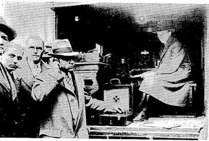
The historical evolution of these level measurements is quite telling in itself. In the 1920s, when electrification allowed an electrical circuit to measure sound levels, the first measurements, done in New York City around 1928-29, were in decibels with no frequency weighting given to the measurements. The first measurements seem to have been done, as shown below, by matching the outdoor noise level in one ear with a recorded noise level in the other ear (since matching sounds that seem equally loud is a relatively easy human ability).
Estimating noise levels, New York, ca. 1928
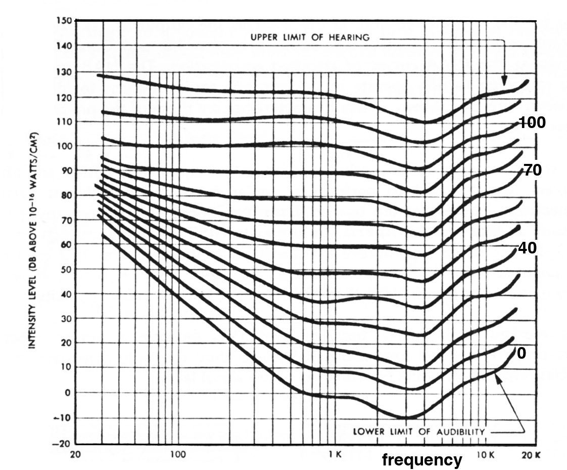
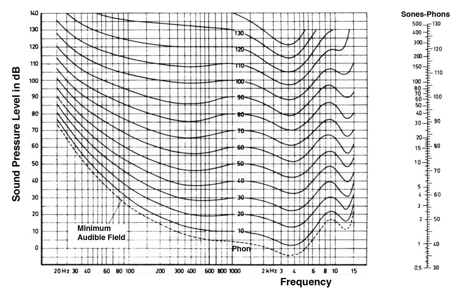
In the 1930s, as introduced in Sound-Medium Interface, the work of Harvey Fletcher and Wilden Munson at Bell Labs produced the original curves of Equal Loudness as shown below (this time right-side up). These curves joined points which represented the dB levels of sine tones (by then a laboratory staple) at different frequencies which subjects found to be “equally loud” in comparisons. Where the curves dipped meant that less energy was needed to sound equally loud to other frequencies that were higher or lower.
Fletcher-Munson curves of equal loudness
Each line also represents a specific intensity level, based on a 1 kHz tone as a reference (note that each dark line approximately crosses a specific horizontal grid at the 1 kHz vertical line). Each curve therefore represents tones that are equally loud as 1 kHz, but which need greater or lesser amplitude to do so. All tones on a line are therefore designated as having the same loudness in phons, which is a kind of hybrid acoustic/psychoacoustic measure.
The overall shape of the curves indicates that at lower frequencies and particularly at lower levels (the bottom half of the diagram) a lot more amplitude level is needed to sound equally loud as 1 kHz (about 12 dB on the 40 phon curve for 100 Hz). At high sound levels, the curves tend to be almost flat, but at lower levels, such as the 40 phon curve, quiet sounds differ a great deal, with basically the lows falling off in loudness, unless sufficiently boosted. The bottom curve, the threshold of hearing, is highly curved. And the range from 1 - 4 kHz always shows a dip, no matter what level is involved, indicating that our hearing is most sensitive in that range.
Listening Experiment. Listen to this short demonstration of the difference in loudness for three tones at the frequencies 50 Hz, 500 Hz and 4 kHz heard in 12 descending steps of 3 dB each. Compare your results at three different listening levels, starting with a normal level for you, and reducing it with each repetition of the example. Count how many of the 12 steps you can hear for each frequency.
Ramps of twelve 3 dB steps at 50, 500 and 4000 Hz
According to the curves, 4 kHz will always sound the loudest and be heard for probably all 12 occurrences, 500 Hz being less, and the 50 Hz tones dropping off the fastest. Was that your experience?
A weighting network: the 40 phon curve (for low levels) measured as dBAStill today, when an acoustical engineer is trying to explain what dBA means to the public, you are likely to hear that it “reflects the way we hear in terms of loudness”. This conveniently ignores the historical fact that the A curve originated for low level sounds (where the auditory system rolls off below 500 Hz), and the engineer is probably talking about measuring higher level sounds found in industry, heavy traffic or aircraft which have a lot of energy below 500 Hz. What happened? Why wouldn’t you use the C-scale (dBC) for such high level measurements?
B weighting network: the 70 phon curve (for medium levels) measured as dBB
C weighting network: the 100 phon curve (for high levels) measured as dBC
The reasons and significance of this evolution towards standardizing dBA measurements are still controversial, but they show how a particular theoretical model, such as the Stimulus/Response model in psychoacoustics, has implications that go far beyond the laboratory and enter the public sphere, in this case standardizing dBA levels for all quantitative by-laws and other regulations.
One argument for this standardization to dBA is that in lab tests, dBA measurements were the best predictor of subjective annoyance (the most typical “response” described in the literature). From a scientific perspective, one would like to have a measurement system that predicts actual subjective findings, but in this case, it leaves some questions still open.
- if the tests were done in a lab, within a context of loudness evaluation, it is likely that the subjects reacted to what they heard, and not to how low frequencies affected the body, i.e. how they were felt, assuming the sounds were reproduced with a realistic bass componentThe Equal Loudness contours were and are an important milestone for the next question tackled by psychoacoustics in the 20th century: loudness, the official subjective response to magnitude.
- low frequency measurement is notoriously subject to “interference” by wind in an outdoor setting, or air conditioning indoors, phenomena that are not normally considered annoying. It is not unusual for a dBC measurement, that is fairly flat in terms of frequency, to be 20 dB higher than a dBA reading in these circumstances. In fact, most listeners are habituated to low frequency sound energy given its prevalence in the sound environment (unless it occurs at high levels)
- from a regulatory point of view, low frequencies do not pose a threat to hearing loss, not nearly as much as the rest of the audible range, and they are extremely difficult to control or abate; however, at high levels for sustained periods, they can affect the body in a variety of ways
Index
C) Loudness. Loudness is the conventional psychoacoustic response to intensity and spectrum of a sound, and as such can be tested with the typical kinds of criteria we have experienced with vibration. First we’ll do a demo of the jnd (Just Noticeble Difference) for loudness.
Listening Experiments. In this example you will hear four iterations of the sequence A B A B with broad-band noise. The second and fourth element in each sequence, B, starts at 1 dB less than element A. Then, after a pause, the difference is reduced to .75 dB, then to .5 dB and finally to .25 dB. Can you hear the difference? Try the experiment at different loudness levels, for instance, start a bit stronger than normal, then reduce it for each repetition of the example.
Loudness Just Noticeable Difference
You probably could tell the difference in the 1st and second groups, but by the third one, it’s getting very difficult, and the fourth group is pretty much impossible to discern a difference. Also, it’s probable that as the overall level got lower, all of the groups became more difficult. The main result you should understand from this demo is that sound level measurements less than .5 dB are irrelevant as there’s no change in loudness that can be heard.
The above chart shows how to add decibels together since they are logarithmic. First you find the difference between the two values to be added, on the top line. This position correlates to the amount to be added on the bottom line. For instance, for equal levels, the difference is zero and the correction is 3 dB. For a difference of 5 dB, the correction is 1.2, added to the higher value.
However, when we realize that the jnd for loudness is around .5 dB, that means any level measurement of a sound that is 10 dB lower than the strongest sound being measured has no appreciable affect on the overall numerical measurement that can be detected aurally in terms of loudness (even though we may well be able to perceive the sound because it lies in a different frequency range). Therefore, keep in mind that Sound Level readings only register the top 10 dB of the component sources that are present, unless there are a very large number of those that are 10 dB lower, in which case we are measuring the top 20 dB sources.
Secondly, we hear three ramps of the same noise, first in 10 steps of 6 dB, then 15 steps of 3 dB, and then 20 steps of 1 dB. Do the steps all sound as equal distances? Would you say that any of them would qualify as “half as loud” for each step? Comparing two stimuli as being equal is relatively easy for subjects to do in psychoacoustic experiments, but to quantify their differences seems less intuitive.
Ramps of 6 dB, 3 dB and 1 dB (Source: IPO4)
You probably found the steps equally spaced, which shows that the logarithmic nature of intensity in decibels is a good choice (a linear amplitude ramp would not sound this even), so just like frequency, logarithmic changes seem to correspond with hearing (except that for loudness, there is no effect like the 2:1 octave relationship found in pitch that seems to repeat the “same” note).
However when it comes to the question, what is twice or half as loud, would 3 dB or 6 dB steps seem to qualify? As noted above in the discussion of the decibel, the 3 dB step is “half intensity” and the 6 dB step is “half amplitude”. Part of the problem here is that you’re listening to abstract sounds out of context (just as we did with sine-waves in the Equal Loudness examples where 10 dB is regarded as a doubling of loudness).
Two different ways to think about the contextual influences are:
(1) the “logical” way, for example if two cars are measured at 70 dB separately, then together they should measure at 73 dB in terms of intensity. You know there’s twice as much energy involved.This next example illustrates this last point with a voice recorded in an anechoic chamber, that is, with no reflecting surfaces and near complete absorption of any reflected sound. The rule here is that there is a 6 dB loss per doubling of distance (also discussed in the next module in terms of propagation). This does not hold for normal rooms where resonance and reverberation prolong the decay of the sound. Despite this, we do have a lot of practice of trading distance with loudness based on environmental experience.
(2) the "perceptual" way, based on your experience with size-distance relationships that we are familiar with in the environment, both visually and aurally.
Recorded voice at difference distances (Source: IPO4)
Loudness Summation. During the 1940s and 50s, S. S. Stevens (known to his students and colleagues as “Smitty”) conducted research at Harvard into the classic Stimulus/Response paradigm that dates back to 19th century psychophysics, as introduced in the Sound-Medium Interface module. He is best known for revisiting the Weber-Fechner law where sensation grows according to the logarithm of the stimulus.
He refined that law in tests for about two dozen forms of sensation, including vision, hearing, tactile sensations of various kinds, pressure, and two other aural cases (vocal effort and duration), among others. For each he established the exponent of the logarithmic relationship, some of which were close to 1 (e.g. vocal effort and duration), and others differed more widely. The exponent he found for loudness was .67, and the entire model became known as Stevens’ Power Law.
Although many critiques have been made of this work, we will show how the process and effect of loudness summation works in the lab, and how it was extrapolated to environmental noise measurement.
The logic behind loudness summation follows from the principles of Fourier Analysis covered in the previous module. That kind of analysis states that a complex tone (fundamental and harmonics) can be analyzed as a set of harmonically related sine waves, each with its own amplitude. In order to determine why a complex tone sounds louder than a sine tone, Stevens followed the same logic, meaning that if you know the loudness of a particular frequency at a given intensity, then you should be able to add the loudness contributions of each of the harmonics to get a sum.
There is one more facet to the approach which is to acknowledge the role of the critical bandwidth in spectral processing. Harmonics that lie within a critical bandwidth need to be summed first and then converted to their loudness contribution. This means that those frequencies lying within a critical band are analyzed for their collective stimulation of the hair cells, not as individual contributions, as are the lower harmonics. There is a complex formula for Steven’s loudness summation in a Handbook Appendix.
By the time Stevens is doing this work, the International Standards Organization (ISO) had issued a revised version (R 226) of the Fletcher-Munson curves with more refined values. The same general shapes of the curves remain, but there is some detail added in the very high frequencies.
Modern Equal Loudness Contours with sone/phon conversion scale (click to enlarge)
Recall that each curved line represents a value in phons, indicating that all points on the curve sound equally loud at that frequency and intensity level. Moreover, the 40, 70 and 100 phon curves in their inverse forms as filters were well established in sound level meters (although the B curve was generally omitted, and dBA was starting to be the universal standard).
However, phon values could not be added, that is, 40 phons + 40 phons does not equal 80, but only 50. Therefore, yet another unit was added, namely the sone, a unit of loudness. The scale at the right shows the conversion from phons to sones, based on 1 sone = 40 phons. As the phon scale increases by 10, the sone scale is doubled. This means that the loudness contribution of each partial in a spectrum, as expressed in sones, can be added together, along with the summation formula discussed above for those falling within a critical bandwidth.
You may have the impression that this is a lot of work just to explain why a complex tone sounds louder than a sine tone – and you would be right! However, as tempting as it would be to leave out this entire historical development as a lab exercise, it has not been treated that way in Noise Measurement. In the module dealing with that subject, we will show that an exactly analogous system for loudness summation of narrow-band noise components (from aircraft engines) was formulated in the 1960s to create the Perceived Noise Level in PNdB.
This came at a time when jet aircraft were being widely introduced with acoustic spectra that had a significant amount of energy in the 1-4 kHz band, where the ear is most sensitive. This had to be taken into account when measuring jet noise, and, more importantly, to predict negative community response at a time when lawsuits were being launched against airports for lost property value – no longer an esoteric lab experiment!
If you’d like to take a few minutes and do a loudness scaling experiment, click here. It’s not so much about the “accuracy” of your judgements, but the fact that you are asked to make them. Is it something you can learn to do (most likely), but is it something that you would actually do in everyday situations (probably less so).
Index
D) Volume. The S/R model can be critiqued for its lack of what is now referred to as “ecological validity”, that is, having a good correlation with the complexity of real-world everyday situations, as distinct from a highly controlled laboratory context. In terms of loudness, that meant one thing to a psychoacoustician of the Stevens school, and quite another to the general public who often were confronted by noisy situations they regarded as “too loud”.
Paradoxically, an alternative approach and terminology was already present, but had been superseded, particularly in North America, by the loudness summation model. That term was volume, and could be found in the literature of the 1920s and 1930s which was strongly influenced by gestalt models of perception.
During that period, volume was regarded as the psychological measure of the magnitude of a sound as perceived, and, more importantly, was regarded, like timbre, to be multi-dimensional. Textbook examples stated that it depended not just on frequency and intensity, but on harmonic content, reverberation, duration and other spatial properties. In other words, it took a holistic approach to perception. However, its failing, which may well have accounted for its demise, was that there was very little scientific methodology to test its properties.
Just as electrification in the 1920s had spawned a whole research methodology based on sine wave oscillators and electrical measurements, it took until the digital era to be able to explore other models and deal with the complexity of sound perception in the real world.
Listening experiment. Let’s start with a simple – but quite dramatic – listening example. This is a comparison of two recordings of shipbuilding. The first is of a man building a wooden boat in France, using traditional skills in a small shed, and the second is of a fairly large steel hulled boat being pounded and riveted in a much larger space in Atlantic Canada. In the audio file, the maximum amplitude for the strongest hit is exactly the same in each recording (-2 dB), and just for the record, so is the RMS value of the first five hits. Yet, there is a vast difference in the sound – which has the greater sense of volume? And why?
Two shipbuilding examples
(Source: WSP Europe 53; WSP Canada 51 take 4)
Click to enlarge
We don’t need to hide the answer as it’s very obvious. The steel shipbuilding conveys a sense of huge volume, compared with the small wooden boat. The factors creating this perception of aural volume are the richness of the steel hull resonances which last longer than the more muted wooden ones, the reverberation in the larger space compared with the relatively dry woodworking shed, and the multiple attacks with metallic tools indicating a strong force for each hit.
Listen to the example a second time at half the playback level. Does the metal ship seem smaller in any way? No, it simply becomes more distant. Just as we know that a small-sized person is more likely to be simply farther away, our auditory experience knows how to distinguish between the volume of the sound and how distant it is, even if a sound level meter couldn’t do that. This type of perception is sometimes referred to as size-distance trade-offs that work with a "constancy of volume".
In other words, in the acoustic world, more effort or force in the excitation function that sets the source into vibration results in a richer spectrum, not just a louder one. However, in the electroacoustic world, added amplification of a sound adds greater loudness, but not the perception of added effort or energy in the source via a richer spectrum. It is highly ironic that the most common use of the term “volume” is on amplifiers, which is exactly what they don’t provide, just loudness!
This “mismatch” in reproduced sound is sometimes merely ironic (e.g. a full orchestra emanating from a small speaker), but the opposite direction – a diminutive sound such as whispering that is close-miked and amplified can be quite striking, psychologically, as it implies a proximity to the source that isn’t physically present. The sense of volume is key to understanding aural perspective in the soundscape.
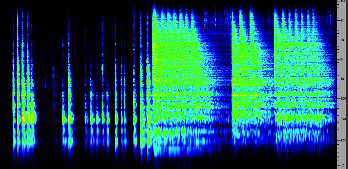
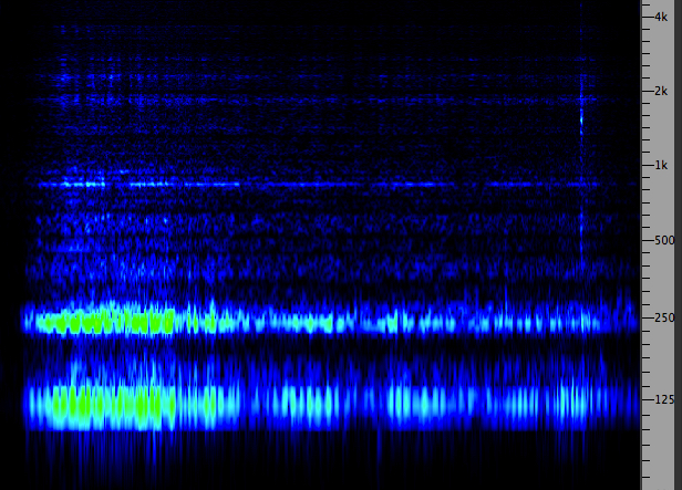
The second example comes from an unexpected source, digitally synthesized grains of sound composed of sine waves by a process called granular synthesis. The example begins with all of the streams of grains in synch with each other, giving the sound a flat dimensionality. After a few seconds, the grains are de-synchronized, and quite suddenly the volume of the sound expands to three dimensions. Then, a further enlargement is made, that of the frequency range from which the grain frequencies are chosen. Finally at the end, the sense of volume collapses as we return to the synchronized version. The spectrogram also gives some visual clues as the sense of volume that is perceived.
Synchronized grains going to unsynchronized
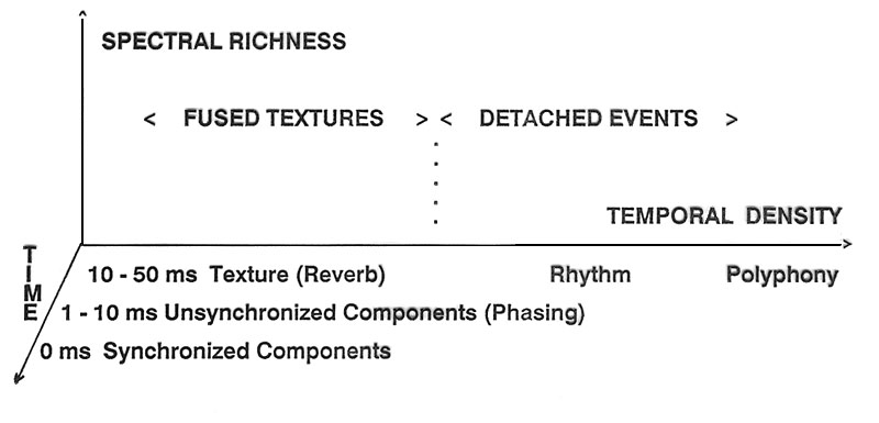
Here is a diagram that attempts to summarize the multi-dimensionality of volume that we have encountered (from Truax, Interface, 21, 1992).The y-axis (spectral richness) and the z-axis coming towards you (time) is exactly what we see in the spectrogram (which is actually 3 dimensions with colour indicating the strength of the frequencies in the spectrum). The added dimension on the x-axis, that we’re calling “temporal density” (because there is no standard term for it yet) refers to the type of unsynchronized and un-correlated components of the sound that can be thought of as constituting a fused texture. At the low end of the time domain are the micro-temporal variations we just heard with granular synthesis, including phasing (in the range of 1 - 10 ms). Then there can be denser, iterated elements that produce a sense of texture, and then all of the reflected sounds coming after about 100 ms that result in a reverberant tail.
The diagram also speculatively suggests on the right side that we might extend this sense of volume to detached events on a macro scale which might describe musical works or complex soundscapes.
In conclusion, the sense of volume of a sound that is described here can be thought of as representing the “space” (and its complexity) inside a sound. The auditory system seems to know how to integrate a variety of spectral and temporal analyses into a coherent image of the complete sound, including a sense of its magnitude which can be expressed as volume. Where loudness is a single dimension, volume is a multiple one.
Index
E) Temporal Aspects of Loudness. In the Sound-Medium Interface module, we introduced the idea that hearing sensitivity is constantly changing with ambient conditions. This is because in louder environments, the hair cells are overstimulated and cease firing, thereby reducing the impression of loudness. Conversely, when we are in a very quiet environment, small sounds seem to be louder than we would expect. The process of this changing hearing sensitivity is called temporary threshold shift (TTS). Therefore, in everyday situations our impressions of loudness are relative, not absolute.The reason for this is that the ear is averaging sound energy over about 200 ms, and the total stimulation during that period is represented to the brain in terms of loudness. Obviously individual amplitude variations in a waveform do not (luckily) create an impression of changing loudness, but only in approximately 200 ms chunks.
However, we should distinguish between two related processes, adaptation and threshold shift. Adaptation is a change in loudness level during a constant sound. Threshold shift is what we are left with after the constant level sound is gone. Both processes involve a decreased impression of loudness, and in the latter case, if the exposure to loud sound has been long enough, we can even feel temporarily “deafened”. Some recovery time will be needed to return to normal hearing.
Loudness also depends on the duration of the sound, with very short sounds such as clicks producing less loudness, even if the energy level is about the same. In this example you will hear seven durations of broad-band noise, starting with 1 second, then decreasing through 300, 100, 30, 10, 3 and 1 ms with some masking noise added. The second sound seems about equal to the first one, but thereafter, loudness will drop off.
Noise bands of decreasing duration
(Source: IPO8)
However, it will be shown in the Audiology module that extremely short peaks or impulses with a high amplitude level can still enter the inner ear and cause damage to the hair cells, without ever being registered by the brain as being particularly loud. You may have experienced this with bottles being hit or sudden metallic impacts; they may not sound very loud, but they can leave a painful sensation in the ears. This problem will be illustrated in the Audiology module.
The terms dynamics or dynamic range are used in various contexts referring to loudness, and should not be confused with the more general use of a similar term such as a “dynamic process”, which usually refers to something unfolding in time. In music, the dynamics of a piece of music refers to its loudness level, which in Western musical practice is usually specified in a general way by Italian terms such as forte (loud), mezzoforte (medium loud), and piano (soft), plus the extremes at both ends, fortissimo and pianissimo. These terms are left to the musician’s sense of appropriateness to the music, and are not absolute in terms of sound level.
In electroacoustic practice, dynamic levels refers to the range of amplitudes within a sound or a recording, from loud to soft, and dynamic range refers to the available amplitude range of a storage or transmission medium. In one of the electroacoustic modules, we will discuss how the dynamic levels of an audio signal will “fit” within the dynamic range of an analog or digital medium, and how to optimize the signal-to-noise ratio of that signal within the medium.
Compression of the dynamic range is commonly used in those situations so that the range of levels from quiet to soft is reduced, and then the overall signal is usually boosted to increase its loudness and improve the signal-to-noise ratio, as well as for other considerations. These include making a sound seem to be actually louder and more consistently louder, with the psychoacoustic result of it being easy to habituate to as an audio environment.
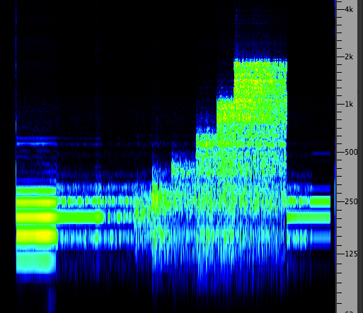
Here is a simple, and somewhat exaggerated, use of compression to increase the loudness of a percussive sound (made with a PVC tube). Since the auditory system does not respond to low frequencies as much as higher ones, it is often difficult to get a strong impression of loudness in them without going over the available dynamic range of a recording (even though subsequent amplification and bass emphasis is readily available).
In this case, the attack sound is strongly limited in level via compression, so that the entire signal can be raised. The graphic at the top shows the power spectrum of the four sounds; the first two are the original, and the second two are the compressed versions, and the bottom part shows the spectrum. Note that the frequency scale only applies to the spectrum.
Low pitched percussive sound, original and compressed
What is remarkable is that listeners barely notice this “distortion” of the dynamic range of the sounds they are listening to, at least not by comparison to poor frequency response that is readily noticed as a degradation of the signal. The prevalence of the practice in audio design may make it seem “normal”, even preferable, and in certain situations, such as a noisy car or other listening environments, the extra loudness makes the sound more audible. Or, given the threshold shifts in our hearing that adapt our hearing to ambient conditions and make loudness a relative impression, we are less likely to notice manipulations of dynamic range.
Index
F. The envelope of a sound. When we refer to a sound’s envelope, we normally mean how its amplitude changes over time. However, keep in mind that in the previous module, we introduced the related concept of spectral envelope, which is how the spectrum of the sound varies in strength over its frequency range. The parallel is appropriate because the auditory system seems to have pattern detection mechanisms for each of these dimensions, frequency and time, and they act in tandem. This will be particularly evident in the module on Speech Acoustics where, in general, vowels are identified by their spectral envelope, and consonants by their temporal one.
The parts of the envelope are usually defined as the attack, which includes onset transients, important for the identification of the sound; the steady or stationary state (even though acoustic sounds are never stationary), and the decay of the sound which includes any reverberation which prolongs its duration.
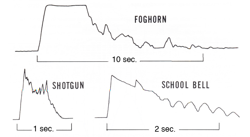
Foghorn Shotgun blast School Bell
These graphic level recordings show that in the foghorn sound, the decay clearly includes the reverberation created by reflections from its surroundings, whereas with the school bell, the longer resonances constitute the decay. With the shotgun blast, this is a very short, powerful sound, and there are some reflections from nearby trees that are so close together that they sound like a single echo.
Sustained acoustic sounds may also have internal dynamics that give them a special character, or in the case of electrically produced sounds, they may seem “flatline” in terms of amplitude such as hums or drones with much less variation than their acoustic counterparts (listen to the examples in these links). Steady sounds like this will definitely result in auditory adaptation in terms of loudness, and only background attention being devoted to them because of their lack of new information.
Power line hum with internal dynamics
(Source: WSP Can 77, take 3)
(click to enlarge)
Index
Q. Try this review quiz to test your comprehension of the above material, and perhaps to clarify some distinctions you may have missed.
home