|
NOISE |
Noise Measurement and Effects of Noise
|
NOISE |
Faced with the daunting task of dealing effectively with this large topic, we can at least rely on the two main parts of the foundation that we have laid with the Magnitude module (specifically the creation of the decibel as the unit of level measurement, and the associated frequency-weighting scales), and the Audiology module where hearing loss has been summarized.
Although noise as a phenomenon and issue can be traced back as far as one wishes to go in the history of civilization, we can arbitrarily date the modern period where measurement and effects of noise became the focal points with the 1929 publication Urban Noise, which reported the results of the first extensive noise study of a major city, New York. Sound level measurements in decibels were used and the Health Department reported a basic set of effects that we can recognize today. You can see some fascinating excerpts, data and even cartoons of the day here.
Since then, there has been a huge amount of research done, and continues to develop, but what has not kept up is what today is often called “knowledge transfer” between the research community and the general public. A forthcoming book by Dr. Marcia Epstein, Living with Noise: A Listener’s Guide, will be a welcome addition to our modest efforts here. These will be our selection of topics.
A) Level measurements today
B) Physiological effects of noise
C) Interference with speech communication and task performance
D) Noise measurement systems specifically for indoor levels, traffic and aircraft noise
E) Noise maps
P) Downloadable pdf summary of Noise effects (control click or right click to download)
Q) Review Quiz
home
A. Level measurements today. Today there are two international standards for sound level measurement, decibels on the A-scale (dBA) and the Leq measurement which is the time-weighted average of acoustic energy, usually weighted on the A-scale as well that rolls off low frequency sensitivity.
The capital letter L, standing for level, is widely used to refer to any set of level measurements in dB, with qualifying letters or numbers to clarify what secondary parameters are applicable. Therefore L stands for a measurement of Sound Pressure Level, that is, an unweighted measurement in decibels.
The qualifiers can be placed as a subscript or in brackets if that is more convenient. Therefore we can refer to LA or L(A), or give a measurement in the form L = 60 dBA, all of which mean the same thing, a Sound Level measurement on the A frequency weighting scale.
As we have discussed several times in the Tutorial, the A-weighting network was originally designed to reflect the auditory system’s sensitivity at low sound levels, according to the Equal Loudness Contours, and we have outlined the arguments for and against their use at all intensity levels here. But the fact remains that all international standards are quoted in dBA.
When we want to measure environment sound levels over time, how can this be expressed, particularly in an urban context where levels can vary quite widely? The logarithmic nature of the decibel means that you cannot average levels arithmetically. On a Sound Level Meter (SLM), the slow response scale already does some averaging over each second in order to provide a single, most typical value. Slow and fast time scales can also be incorporated into the measurement unit as an S or F, respectively.
However, when the overall levels in a soundscape vary widely, it would be very misleading to do any averaging. As an extreme example, consider levels of 20, 50 and 80 dB. If these were made on a linear scale, then you could say the average is 50 dB. But they are not; in fact, the ratio of 80 dB to 20 dB is a million to one, and from 80 to 50 is a 1000 to one, so clearly it makes no sense to average those values.
Instead, sound levels can be reported statistically, in terms of what percentage of measurements exceeds a certain level. Here are the most common instances:
L10 the level exceeded 10% of the time, namely the peak levelThere are sometimes references to L1 and L99 for the extreme values at the high and low ends, but these are clearly singular cases and not representative, whereas the peak and ambient levels referred to are more typical and useful.
L50 the level exceeded 50% of the time, the average or mean level
L90 the level exceeded 90% of the time, namely the ambient level
One word of caution, the norm for this data is that it is the level that is exceeded but occasionally an author will quote the opposite – not illogical but potentially very confusing.
Note that L90 - L10 can represent the dynamic range of the environment. If this is very small, then the levels are very steady and hence more likely to be promote adaptation in the listener (and sound pretty boring).
Equivalent Energy Level Leq. The solution to the problem of averaging decibels noted above is to tally the actual energy being experienced over a certain time frame, before converting it to the logarithmic decibel. As such, this is a useful measurement of dosage (i.e. energy plus duration).
Another way to think of the Leq is that it represents the same constant amount of energy as if it had been experienced over the same length of time, hence the reference to “equivalent”. It is usually A-weighted and indicated as LAeq.
Just to complete the simple example of averaging 20, 50 and 80 dB, the result would be Leq = 75 dB, which seems much more reasonable. Also, note that the Leq value is not equivalent to L50 unless the dynamic range is very small (as in the visual averaging of nearby levels). The Leq method recognizes the large differences in intensity that are present in higher dB levels.
The total duration for a Leq measurement needs to be indicated, such as a 24-hour measurement Leq(24) which gives a comprehensive accounting of how much sound is being experienced for an entire day. A variation on this, called the Day-Night Equivalent Noise Level, gives a 10 dB boost to the nighttime levels between 2200 and 0700 (10 pm to 7 am) in recognition of the added risk for sleep disturbance, and is symbolized as Ldn or DNL.
Leq and Ldn have been used for global risk criteria such as:
Leq(24) = 70 as the noise exposure threshold for hearing damageHowever, correlation of exposure levels with annoyance is extremely difficult as it depends on such factors as the relation between the person and the noise maker, individual listening habits, education and life style, attitudes towards the necessity or preventability of the noise (including opinions as to the intentions of the noise maker), previous noise exposure, and the means available for complaint.
Ldn = 55 as the threshold of expressed community annoyance, which has been found to be the level for which 17% of the population will express a high degree of annoyance.
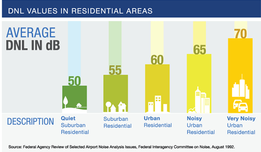
The Federal Aviation Agency (FAA) has adopted a DNL level of 65 dBA as the threshold for “significant noise exposure”, or the equivalent in the CNEL system in California (see below), although it is unclear what this means in practice.
24-hour DNL levels for various residential areas (Source: FAA)
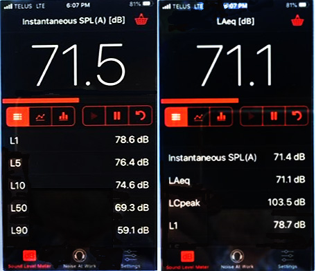
Today one can get an inexpensive app for a smartphone that has most of these measurement options readily available, such as the NoiSee app shown here. In the photos below, we see two typical displays. On the left is an instantaneous dBA measurement that tracks dBA levels in real-time mode. Beneath it are the L10, L50, and L90 values accumulated since the last reset. On the right is the cumulative Leq value in the top window. It is quite interesting to watch the display and see how it correlates with what you are hearing.
A word of caution: these levels on a smartphone app will not be precisely accurate if a calibration procedure has not been done. However, for the kind of pedagogical purpose we have in mind, they are definitely close enough to give you a good idea about sound level measurement and your degree of noise exposure.
These readings were taken over a 4 minute period on a main urban thoroughfare after the rush-hour with a medium density of cars. However, there were also several buses and one large truck which accounted for the highest levels. The peak of the C-scale reading at 103.5 dB looks very high, but that simply reflects how much low-frequency energy there is in a typical traffic ambience.
Index
B. Physiological effects of noise. The effects of noise are generally divided into sub-categories such as physiological, psychological, sociological, and particular types of activities such as speech communication and task performance. While the psychological and sociological effects of noise are very significant, they are also far too extensive (and depressing) to be dealt with in this format. Since many of them begin with more basic physiological effects, all of which intertwine in terms of health and cognitive development, we will emphasize those in this section.
The physiological effects are largely involuntary responses of the body, and the main effect here is that noise is a stressor on the body leading to hypertension. We often think of stress as a psychological state, but there are direct, bodily effects as well.
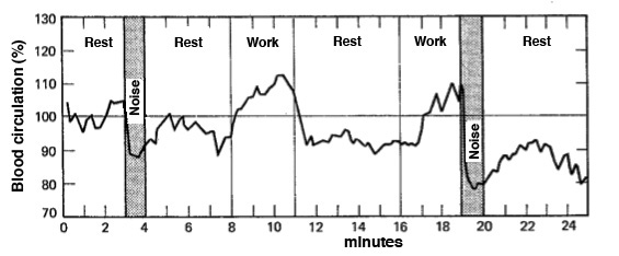
Breathing rate can increase, as can skin resistance and muscle tension. However, the one that has a significant effect in terms of sound is blood circulation which is the inverse of blood pressure. In this diagram we can see how blood circulation can rise during work activity, recover with rest, but decrease with noise exposure.
The reason is vasoconstriction, a narrowing of the blood vessels when the smooth muscles in the blood vessels tighten and narrow the opening, thereby increasing blood pressure and lowering circulation. The opposite affect is vasodilation, a widening of the blood vessels.
Blood circulation during noise, rest and work (source: White)
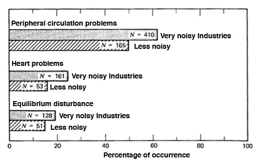
Why this is important is that the blood supply to the hair cells is diminished, and the result is TTS, a temporary threshold shift. Of course, if deprived of nutrients for a long period of time, the hair cells can die. This condition can also result in dizziness because of the connection to the semi-circular canals of the cochlea, and a cold feeling in the hands and feet, the “extremities”. These types of problems have been documented with workers in noisy industries as shown here.
We have now established a link between noise, stress and blood circulation, and connected it to hearing loss, as summarized in the Audiology module, which is the best understood aspect of the physiological effects of noise. However, the same cannot be said for noise-induced sleep disturbance.
Physiological effects in noisy industries (source: White)
Sleep disturbance. The effect of noise on the disturbance of sleep has been known, as least anecdotally, for some time – it was one of the effects cited in the 1929 New York study referred to above – but what has changed since then is our understanding of how noise can disturb the sleep level, raising it from a lower state to a higher state without the person waking up.
The different levels of sleep are categorized by stage I and I-REM (the rapid eye movement stage associated with dreaming), through the lighter sleep level of stage II, and then the deeper levels (III and IV, which are now usually combined), and back again in a cycle. A good sleep pattern will have about 4-5 cycles of this pattern. We now know that even a single sound, such as a passing car or truck, can cause a change of sleep level towards a lighter state, and since the person has not woken up, there will be little awareness of the effect.
However, there can be an after-effect in the sense that one hasn’t “slept well” or “didn’t get enough sleep” – a little like a hangover (which also prevents the deeper levels of sleep from occurring) – and these effects can manifest themselves in reduced task performance or mood changes the next day.
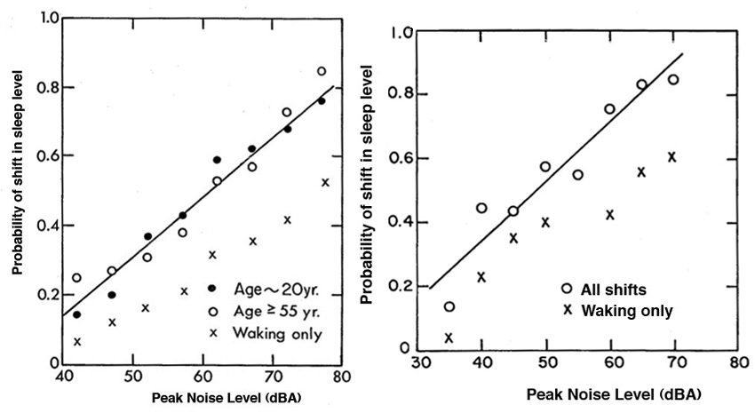
The data on this subject is not entirely in accord with each other as to the variable of age differences, but the general pattern is that a shift in sleep level is about twice as likely as an event that wakes the person, as shown in this Canadian data. Subjects were exposed to different levels of recorded truck noise seven times per night, and the data shows the probability of a shift in sleep level, or waking, for a single truck passing.
Most studies show that children and younger adults are less likely to experience this kind of sleep disturbance, but there is variability in results for middle-aged and older subjects; in the above case at right, the former are reported as being more likely to be disturbed. However, all data shows that a shift in sleep level is more likely than waking.
Probability of a shift in sleep level versus waking, in younger and older populations (left), and middle-aged subjects (right)
(source: Thiessen)
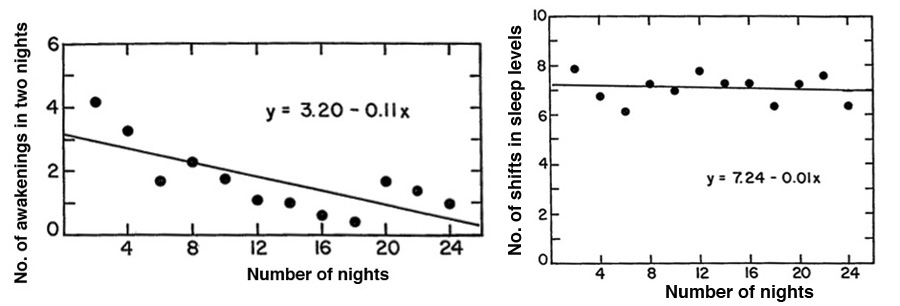
The question of habituation to noises during sleep is often poorly understood by the public. People report that noises that once woke them up (for instance, in a new living space context) can be habituated to over time, and that is backed up by the next graph at the left in terms of fewer instances of waking. However, the “bad news” people are not generally aware of, is that there is never any habituation to shifts in sleep level (which, again, is something one is not aware of), as shown in the righthand graph.
In fact, all involuntary physiological reactions found in the sympathetic nervous system (best known for the so-called "fight or flight" reflex) seem to have this property. And, in the case of sleep, these lighter sleep levels do not allow the blood pressure variations to follow their normal circadian rhythm.
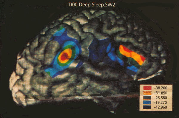
We also know that multiple areas of the brain are stimulated by incoming auditory stimulation, even during sleep. The following PET scan shows activity in at least two areas, the auditory cortex and the frontal lobe which controls executive functions such as attention and motor functions.
Probability of waking to seven noises of 65 dBA over 24 successive nights (left), or a shift in sleep level (right) (source: Thiessen)
In this case, the brain is responding to tones while in a deep state of sleep. We've all heard the anecdotes about a mother being wakened to her baby’s cry, or some similarly salient sound, and here is the modern understanding of that phenomenon. The brain can habituate to known sounds, and determine their saliency, even during sleep, as to whether "waking" is needed.
PET scan of brain functions during sleep when exposed to tone stimlationQuestion: Have you ever heard someone say that when they went on holiday somewhere new, they “couldn’t sleep because it was too quiet”? Does this mean that a quiet ambience for sleeping is not a good thing? Answer here.Given this data about sleep, not to mention how much general health is dependent on it, recommendations for optimum sleeping conditions vary from less than 35 dBA to less than 45 dBA, but in general, the quieter the better. This brings up socio-economic issues, as poorer neighbourhoods often have less adequate sound insulation, greater density of people, and fewer restrictions on car and truck noise at night. If you’re a student (or anyone else for that matter), think about this before you rent or move!
Index
C. Interference with speech communication and task performance. There are various approaches to measuring speech intelligibility, some based on standard hearing tests, and some focused on particular environments with differing levels of noise.
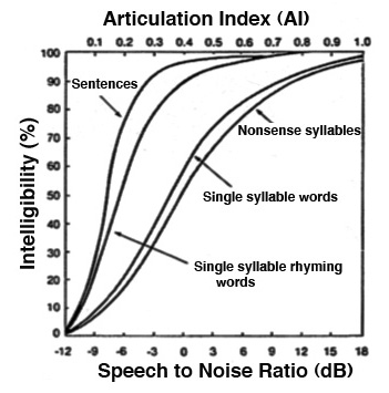
The Articulation Index is a general measure, ranging from 0 to 1, for the percentage of words or speech elements that are correctly recognized in a particular context. This may be judged by the simple exercise in a standard hearing test where a single word is spoken via headphones in each ear separately at progressively lower intensity levels (similar to pure tone audiometry). In other cases, a level of background noise may be added, which somewhat replicates the more typical environmental situation where a person with hearing loss has trouble distinguishing speech in a noisy environment, as covered in the Audiology module.
An AI value above 0.7 (70%) is regarded as good intelligibility, and below .3 (30%) very poor. We can get a general idea of how the AI value relates to the speech-to-noise ratio in dB and overall speech intelligibility in this diagram for sentences and various words or syllables. Notice how rapidly intelligibility falls off when the speech level is lower than the noise level, and conversely how speech needs to be around 9 dB higher than noise for good intelligibility (assuming normal hearing).
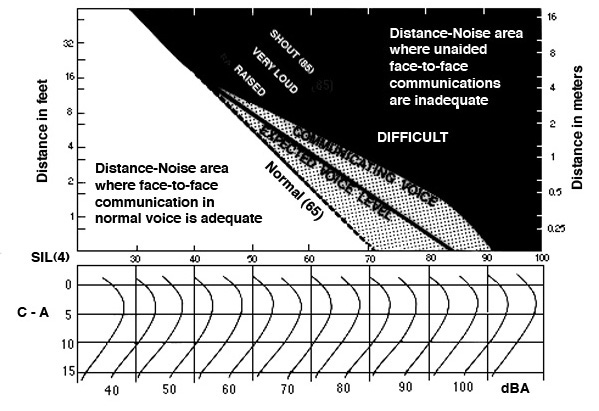
The Speech Interference Level (SIL) system has also been developed to correlate with various ambient conditions and the distance between speakers in applied settings. The main measurement is the average of the spectrum intensity in the four key speech band octaves: 500 Hz, 1 kHz, 2 kHz, and 4 kHz (although other bands such as 3 kHz and 6 kHz may also be integrated in related tests). The average of these values is called SIL(4) as shown here.
If we assume 6 feet (2 m) as an acceptable “social distance”, then a normal speech level (65 dB) can be understood when the SIL value is 50 dB or about a 65 dBA overall level. For levels above that a raised voice is required, and if the communication is “vital”, then a projected “communicating voice” is needed. There is also a typical gender bias built in here, as most of the tests have been done with male voices.
The Speech Transmission Index (STI), developed in the Netherlands and used primarily in Europe, includes all octave bands between 125 Hz and 8 kHz. Further refinements with these systems have been made for “rapid speech” and for particular contexts such as public address systems, telephone and telecommunication systems.
For telephone conversations, an ambient level of 60 dBA or less is regarded as adequate, and above 75 dBA as unsatisfactory, with a raised voice required in between.
Task performance. We will summarize the main effects here in point form with some commentary. The general issue is the degree of "cognitive load" involved with the task, those that require concentration and logical analysis being more susceptible than those that are repetitive (in which case, it is known that adding background music will likely increase productivity and worker satisfaction).
- steady noises do not interfere with performance unless > 90 dBA (depending on the complexity of the task; for instance, multiple ongoing tasks will be more affected)These last two points refer to social behaviour. The first about the lack of “helping” refers to some much publicized studies about subjects being less willing to assist someone (even when they were obviously physically impaired by an arm cast, for instance) in the presence of noise. Others recommended lower salaries for fictitious employees when exposed to 70-80 dB noise levels (remember that if you are a teacher involved with grading).
- irregular (unpredictable) noise bursts are more disruptive than steady noises
- high frequency components above 2000 Hz interfere more than low frequency components
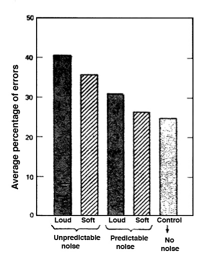
Source: White
These results shown at the left are for a proofreading task, one that requires focus and concentration, with and without noise, with two secondary variables as to whether the noise is loud or soft, unpredictable or predictable. There are many such experiments that have been done for various tasks, but this one captures the general pattern of the possible interference by noise.
Basically it shows that louder noise is more stressful and tension producing, as we saw above, and that the brain can habituate to steady or predictable noises. Unpredictable noises by their very nature are distracting and can cause one to lose focus. Something similar can happen with music as a background, depending on how "predictable" it is.
- noise does not influence the overall rate of work, but may increase the variability of the work rate
- noise is more likely to reduce the accuracy of the work than the quantity
- complex tasks are more likely to be adversely affected than simple tasks
- may affect decision making and produce momentary lapses in efficiency
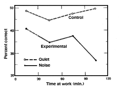
Source: WhiteThis study compares the percentage of correct responses on a “decision-making” test, with questions similar to an IQ test, in relative quiet versus intense noise.
Typically, it shows that this complex task is affected quite seriously by the noise. Other similar tests show a slightly less expected result that it is not the overall quantity or rate of work that suffers, but rather the accuracy of the work and its steady progression. In other words, frequent distractions or stress impair one’s ability to follow through on something more complex, maintain attention and focus, and make decisions.
- children learning in noisier classroom environments perform more poorly than in quieter ones
- immediately after a loud sound (startle reaction), efficiency may drop for a few seconds (the well-known "fight or flight" reaction of the sympathetic nervous system that reduces blood circulation)
- the effects of noise may be felt as an after-effect, such as reduced tolerance for frustration
- background music will improve productivity and morale, particularly with boring, repetitive jobs
- social behaviour (e.g. helping, evaluating) are adversely affected
- subjects who have perceived control over noise show greater tolerance for frustration, even if the control is not exercised
The final point about perceived control is most relevant for dealing with everyday ambient stressors, including noise. This refers to chronic background conditions that are negatively valued, intractable, non-urgent, perceptible but generally unnoticed. A typical case is traffic and aircraft noise that is ongoing, as opposed to a sudden “toxic” event (e.g. runaway house or car alarm) that draws negative attention and annoyance.
The mediating factors to one’s response include a cognitive appraisal of the situation and whether one has perceived control over it. In other words, the mind intervenes to influence one’s reactions. Personal context, such as vulnerability, resources (or lack of them), and experiential factors such as personal salience, past history and personality may also be involved.
In outlining the above issues, Joan Campbell (in Environment and Behavior, 15(3), 1983) discusses both adaptation and coping strategies. Adaptation to the stressor can include cognitive adaptation and a reappraisal of it as benign or tolerable, a diminished motivation to escape or avoid, and less attention being paid. The probability of instrumental responses will likely diminish over time.
Coping strategies involve direction action, information seeking, or palliative coping mechanisms, as well as restructuring one’s relation to the stressor by acting on it directly, or its context, or on one’s own reactions.
Even though this summary has been selective and highly condensed, it hopefully will give a sense of the complexity and intricacy of physiological, psychological, cognitive and social relationships that are involved.
Index
D. Noise measurement systems specifically for indoor levels, traffic and aircraft noise. Many systems have been proposed by acoustical engineers that are designed to apply to specific situations and types of noise. They all include the establishment of what are “acceptable” levels for those situations, which leaves open the question of “acceptable by and for whom”. As such, they reflect the social, economic and political values of the time, and even if superseded, remain interesting in that regard.
Indoor ambient levels. Systems such as the Noise Rating (NR) and Noise Criterion (NC) models were early attempts (1950s and 60s) at establishing criteria for indoor ambient noise levels, particularly in the context of air-conditioning units become prevalent in office towers and related work spaces, thereby increasing their ambient noise levels. On the other hand, there are multiple types of spaces designed for different activities, including residential, and so what is regarded as optimal in one area may be inappropriate for another.
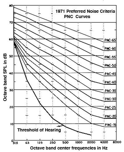
In 1971, Leo Beranek (of the large acoustical consulting firm of Bolt, Beranek and Newman, BBN) proposed the Preferred Noise Criterion (PNC) system for ambient indoor noise levels, which updated his earlier NC values, particularly in response to the low-frequency component produced by air conditioning. The PNC curves were based on the octave-band spectrum analysis of the broadband ambient noise, as shown below, and generally reflect the Equal Loudness Contours.
The subjective component was phrased as “which the occupants find satisfactory”. In the context of steady background noise to which listeners routinely habituate, it is unclear how that could be determined, particularly since the physiological effects, as outlined above, are largely involuntary. Did it simply mean lack of complaints? Issues with speech communication, as discussed above, generally involve higher levels before they pose a problem. Also, steady background noise is unlikely to mask sounds with a sharp attack such as telephone rings or typewriters, or general background conversation.
The PNC criteria for different types of working spaces is reflective of the social hierarchy of business and professional enterprises. For instance, it is surprising that “secretarial spaces” would be grouped with “lobbies, laboratory and engineering” spaces. Fortunately, dBA equivalents were given as well as PNC values, so these values could be referenced elsewhere more generally.
CONTEXT
PNC
dBA
Excellent listening conditions
less than 20
less than 30
Sleeping, residential, private office, library and classroom spaces
25-40
34-47
Large offices, stores, cafeterias and restaurants
35-45
42-52
Lobbies, laboratory, engineering and secretarial spaces
40-50
47-56
Maintenance, equipment, kitchen and laundry rooms
45-55
52-61
Shops, garages, power-plant control rooms, etc.
50-60
56-66
Recommended levels of ambient noise for various indoor spaces (source: Beranek 1971)
Traffic and Aircraft Noise. Today, the standard measurements discussed above, dBA and Leq, also A-weighted, are now what are used pretty much universally for the ubiquitous issues of traffic and aircraft noise.
However, in the past, specific rating systems were proposed and tested in terms of their correlation to subjective factors, generally termed annoyance. The British systems were the Traffic Noise Index (TNI) and the Noise and Number Index (NNI) for aircraft. The latter was originally devised by the Wilson Committee on Noise (1963) as a response to the expansion of Heathrow Airport in London.
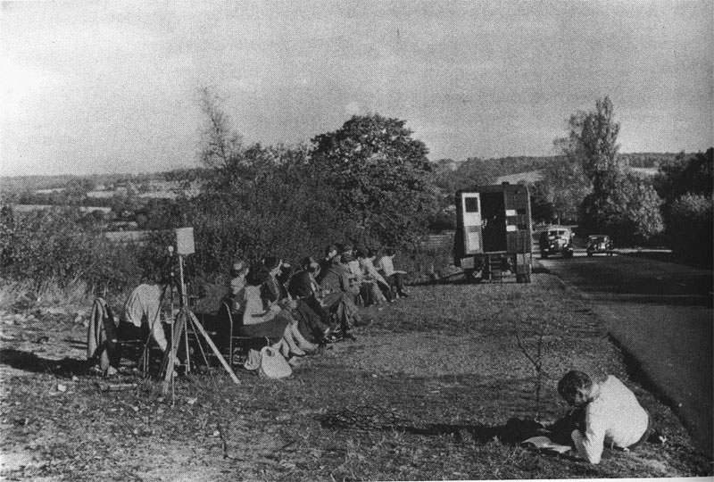
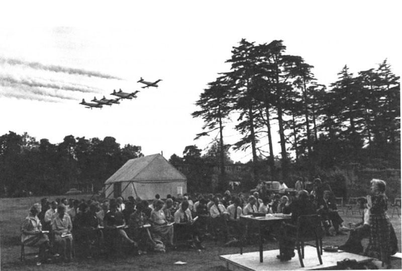
What was somewhat unique in the establishment of the subjective responses and criteria was the use of on-site testing by trained listeners, as can be seen in these photos. The scale used was probably that reported in the NNI diagram below as the Farnborough experiment scale.
On-site subjective evaluations of traffic and aircraft noise in the UK, ca. 1960 (click to enlarge)
The Traffic Noise Index, TNI, is computed from the formula:
TNI = 4 . (L10 - L90) + (L90 - 30) (dB)
What this means is that the dynamic range of the traffic levels (L10-L90) is weighted by a factor of 4, added to the amount of the ambient level above 30 dB. Therefore a more variable range with strong peaks, typical of trucks, would score higher than a steady flow of cars, as would a higher overall level caused by density of traffic. These values were then correlated with social surveys in terms of predicted annoyance levels.
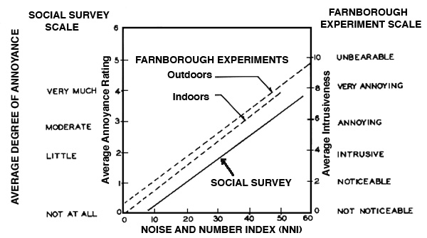
The Noise and Number Index, NNI, formula is based on the Perceived Noise Level in dB (PNdB) that will be explained below, plus the number of flights N, with 80 subtracted because no annoyance was found to be reported at or below that figure. The formula is as follows:
NNI = (Average Peak PNdB) + 15 (log10 N) - 80
As we have seen before, the results of this kind of study are the classic Stimulus-Response model where response is found to increase linearly (on the vertical axis) when the stimulus increases logarithmically (on the horizontal axis).
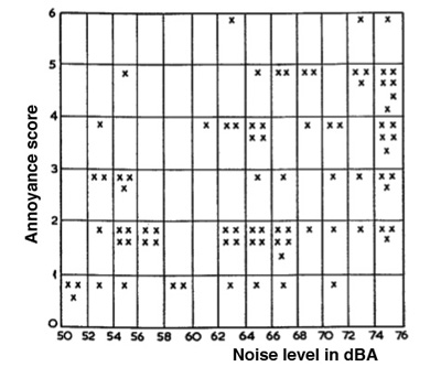
There are at least two problems with this methodology: (1) “annoyance” at different levels is the only type of response being measured, and that in an experimental context (even if on site); (2) actual responses from the general public are more likely to range across a wide “scatter plot”, as shown below, the nature of which is lost in the averaging procedure reported here.
Although researchers who have conducted social surveys will not be surprised by this “scattering” of responses, many of us may be, because in the above plot, we can see outliers who are fairly high on the annoyance scale at levels below the conversational level of 60 dBA. As well, there are below average levels of annoyance reported by others at levels above 75 dBA.
Individual response scores as a scatter plot (source: Tempest)
Clearly there are other psychological and sociological factors involved, some of which were discussed above. The variables are many, including gender, level of education, economic status, as well as those already mentioned.
Aircraft noise and the Perceived Noise Level. A good account of the historical (and political) development of noise legislation for Europe and North America is provided by Karin Bijsterveld in her comprehensive Mechanical Sound (MIT Press, 2008). Here we we summarize one of the most significant cases that originated in North America, the development of the Perceived Noise Level (PNL) system by Karl Kryter in 1959.
The impetus for its development was, first, the introduction of jet aircraft in the late 1950s and early 60s. The engines of these planes had high powered rates of rotation and thrust that resulted in more high frequency energy in the range where the ear is most sensitive, namely 1-4 kHz. As a result they were noticeably louder and more annoying than propeller planes, whose energy was more evenly spread across the spectrum.
Secondly, land use around airports was becoming increasingly controversial, and in fact the first lawsuits around Los Angeles airport were already being launched. The Federal Aviation Agency (FAA), as it still is today, was in charge of establishing appropriate regulations.
Kryter followed an equivalent of the traditional approach we outlined in the Magnitude module to use the Equal Loudness Contours for hearing sensitivity for pure tones (in phons), convert them to a loudness value (in sones), add them together in an appropriate manner. He then converted his result back into decibels, called the PNdB level – the Perceived Noise Level in decibels. Note that the word “perceived” in this case only refers to the auditory system’s response patterns, not to any subjective, environmental experience.
In others words, Kryter substituted noise bands in the PNdB method for sine tones because the spectrum of jet aircraft was the issue. We can trace the historical roots of this additive approach back to Fourier Analysis where a complex tone with many harmonics can be expressed as the sum of sine waves, and the cumulative loudness is the sum of their individual subjective loudness. But in this case, we’re not dealing with just an esoteric lab experiment, but a serious environmental problem with enormous political and economic implications.
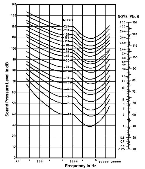
The following diagram illustrates the contours of perceived noisiness he proposed, and which received approval from the International Standards Organization (ISO). They of course resemble the Equal Loudness Contours for sine tones, in always dipping between 1-4 kHz, but instead, they refer to octave noise bands with equal loudness.
Instead of the curved lines representing phons, he needed a new unit of loudness, and so he invented the noy – thereby injecting the subtle humour associated with its plural “noys”. Admit it, we have to like him just for that! This is not a topic noted for its potential humour.
The scale shown at the right of the diagram, the noy compared to PNdB, is exactly analogous to the relation of the sone to the phon: 1 sone = 40 phon and 1 noy = 40 PNdB.
Phon = 40 + 10 log2 (Sone)
PNdB = 40 + 10 log2 (Noy)
By using this traditional additive approach, the PNdB takes into account the spectrum of the noise much more specifically than the dBA measurement, which simply rolls off the low frequencies. The summation method used typically results in PNdB values being higher than dBA by about 12 dB. So, a 100 dBA aircraft measurement will likely be around 112 PNdB. However, PNdB requires computer calculations, and was not available on the Sound Level Meters of the day.
Extensions to the PNL. Not surprisingly, given the stakes and complexity of the problem, extensions to the basic PNdB were created, as we already saw with the Noise and Number Index in the UK, as above, which added the number of flights.
In the U.S., the first extension was to include flyover times and a correction for whistling pure tones, typical of jet engines, which are found to be particularly annoying. This was called the Effective Perceived Noise Level (EPNL).
The EPNL measurement is based on the following equation:
EPNL= PNLmax+ 10 log (t10/20) + F (dB)
where PNLmax is the maximum Perceived Noise Level during flyover in PNdB, t10 is the duration (in seconds) of the Noise Level within 10 dB of the peak PNL, and F is a correction for pure tones (which are generally found to be more annoying than broadband noise without perceived tones). In practice, F is about +3 dB.
Then, in order to predict community annoyance (along the same lines discussed above), a much more comprehensive measure was made, called the Noise Exposure Forecast (NEF), based on the following equation
NEF = EPNL + 10 log10 (ND + 16.7 NN ) - 88 (dB)
where EPNL is the energy mean value of the EPNL Effective Perceived Noise Level and ND and NN are the number of flights during the day (0700 to 2200) and night (2200 to 0700) respectively. The factor 16.7 represents a 10-to-1 weighting of night flights over daytime ones.
Land use criteria (with implications for housing and financing) were also established. For instance, a residential area should have a NEF of 30 or less; between 30 and 40 NEF is stated as suitable for multiple family housing, although it is not clear why a higher tolerance level should apply in this case; above NEF 40, the area is suitable for industrial and recreational purposes only.
Perhaps in reaction to the complexity of the PNdB based systems, the state of California in the early 1970s introduced the Community Noise Equivalent Level (CNEL) which was based on simple dBA measurements. Another difference was that evening flights (1900 to 2200) – a very nice California touch – were given a weighting of 3, along with the standard 10 for night events.
The total noise exposure per day (CNEL) is calculated from the equation:
CNEL = SENEL + 10 log10 (ND + 3NE + 10NN) - 49.4 (dB) where ND, NE and NN are the number of flights during the day (0700 to 1900), evening (1900 to 2200) and night (2200 to 0700) respectively, and SENEL is the energy mean value of the single event noise exposure level (also called SEL) which may be calculated from the equation:
SENEL = NLmax+10 log10tea (dB)
where NLmax is the maximum Noise Level in dBA and tea, is the effective time duration (in seconds) of the Noise Level (on the A scale) and is approximately equal to one-half of the duration during which the Noise Level is within 10 dB of the maximum.
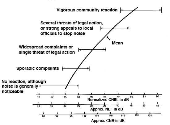
This still sounds complicated, but it could be derived from flight data and Sound Level Meter readings. What is more interesting in terms of response prediction – and very American in its emphasis on litigation and community unrest – is the correlation of CNEL levels with community response, as well as other measurement systems (NEF and CNR). The vertical axis speaks for itself.
Equally interesting, and you can peruse this in the CNEL link, are the “correction factors” that can be added or subtracted from the CNEL values to reflect local community contexts, such as seasonal variation, residual outdoor noise levels, previous exposure and community attitudes (including relations with the noisemaker).
Since that period of rapid evolution (and extreme complexity) in aircraft noise measurement, the aircraft themselves have become less noisy, the FAA has switched to DNL measurements or a California style dBA levels – and yes, those lawsuits in L.A. and elsewhere were successful.
Index
E. Noise maps. Over the last few years, many different kinds of noise maps have been created, often colour-coded to show sound level measurements throughout a city or region (they have become mandatory in EU countries). The time element, however, is problematic both to collect levels at different times of day or longer, and how to display them. The WSP’s early isobel maps that can be seen here showed the contours of equal levels, and were most successful when the time frame was one where levels were relatively steady, such as late evening.
These noise maps can be distinguished from sound maps, which are usually designed so that recordings from particular locations (and times) can be posted according to their location on a map. A web search of both noise and sound maps will provide many examples. Presumably their aim is to draw attention to noise and the soundscape as a whole through a visual medium, perhaps aided by sound examples. However, can they go farther than that?
One particularly good use of maps to communicate large-scale change are these maps illustrating what are called “tranquil areas” in England, comparing the early 1960s to the early 1990s. A separate definition was provided for what constitutes a “tranquil” area, but it is the instantly clear degree of change that is most impressive, for both the country as a whole and the dense area around London.
Click to enlarge
Of course the choice of green to mark the tranquil areas is appropriate, not just because it symbolizes the natural environment, but because “England’s green and pleasant land” is a key phrase from William Blake’s poem Jerusalem that is often regarded as England’s national anthem. As such, it will likely resonate more with English people.
Index
Q. Try this review quiz to test your comprehension of the above material, and perhaps to clarify some distinctions you may have missed.
home