Before
we proceed to the more applied topics of Speech Acoustics,
Audiology, and Noise Effects and Measurements, there is one more
theoretical area to consider. That is the straightforward ways
in which sound waves combine acoustically, and the fascinating
ways that the auditory system practices to separate the
composite sound waves that arrive at our ears into identifiable
sources and what is usually called an auditory stream.
This latter topic is still open-ended in that it involves
cognitive functioning that continues to be researched. It also
involves some basic psychoacoustic processes that are quite well
understood and play a role in everyday perception.
We then conclude with a continuation of the Acoustic Space
concepts that were summarized in Sound-Environment Interaction,
and extend them to the development of the acoustic community
concept, and the Acoustic Niche Hypothesis (ANH).
We will cover these topics in the following sub-sections.
A) Superposition of sound
waves
B) Masking and critical bandwidth
C) Non-linear combination
D) Auditory fusion and streaming
E) Cognitive processing and hemispheric
specialization
F) The acoustic community and the Acoustic
Niche Hypothesis
Q) Review Quiz
home
A. Superposition of sound waves. The most
basic aspect of sound combination is the Law
of Superposition which refers to the linear
addition of two or more sound waves, a principle which holds
in most actual cases. However, since sound waves are
oscillations, containing what might be thought of as positive
and negative parts (representing positive and negative
pressure, or in the case of an audio signal, positive and
negative voltage), simple addition can result in reinforcement
(+ with +, - with -) or cancellation (+ with -).
Reinforcement is also called constructive interference,
and cancellation can be called destructive interference.
Note that the term "interference" does not have any negative
connotations, but rather is a general term for how sound waves
combine.
This process of superposition can be regarded as linear
because it is like algebraic addition, where the term
“algebraic” refers to what was just mentioned – the
positive/negative values of the wave at each instant combine
according to their + or - values, e.g. 5-3=2. The more
troubling issue that arises from the Law of Superposition
is that there is no inherent limit to how large a sound
wave can grow. In the medium of air, linear addition can
theoretically increase indefinitely, hence there is no natural
“limiter” to sound levels. However, non-linearity can occur in
psychoacoustic processing, as will be discussed in the next
section.
We have already had two simple examples of the Law of
Superposition back in the first Vibration module, so we will
repeat those videos here: (1) creating a standing
wave in a string as the sum of two waves traveling in
opposite directions: (2)
adding harmonics together to form a pitched tone with a
richer timbre, and greater loudness than a simple sine tone.
Always keep in mind that sound wave combination occurs all the
time, but we are unaware of it, other than our ability to hear
multiple sounds at the same time. An alternative way of
expressing the Law of Superposition, is that two or more
waves can travel simultaneously in the same medium by their
linear combination. Only in some very particular
circumstances does the “interference” pattern become
noticeable and audible, because of some regularity in the
difference between two waves, for instance.
Three results of interference can be easily observed: spatial
cancellation or dead spots, frequency cancellation or
phasing due to small time delays, and cancellation
between waves of nearly identical frequency, resulting in beats.
Let's look at each of these in turn.
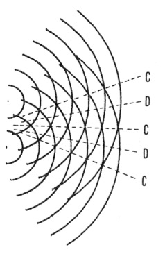
Constructive and destructive interference
patterns are probably most familiar with the visual examples
of water waves because the patterns are readily visible. Take
the classic example of two similar stones dropped into a pool,
from which waves spread out and interact with each other.
Peaks and troughs (the equivalent of the positive and negative
pressure parts of a sound wave) reinforce and cancel each
other in regular patterns.
These patterns are readily seen in a 3-dimensional
representation at right, but they can also be traced in the
two-dimensional version at left with the C and D lines for
constructive and destructive interference where the peaks are
indicated by lines, and the troughs by the empty spaces in
between.
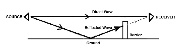
With
sound, we encountered destructive interference, for instance, in
the ground effect described in the Sound-Environment
Interaction module, where it referred to the attenuation
of sound between the direct and reflected wave.
But there is
no audible pattern involved here that is similar to the water
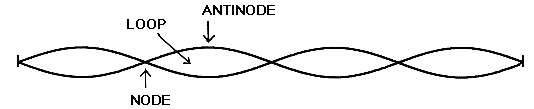
waves. For that to be experienced, as we also did in that module, we need an
enclosed space where standing waves (heard as pitched
eigentones) are created. Positions of minimum sound pressure
called nodes or dead spots can be experienced in
a standing wave, along with pressure peaks called antinodes.
These can be experienced because they are stationary, not
constantly changing as they would be in an outdoor situation.
16. Personal Listening
Experiment: Find an enclosed space where there
is a steady drone sound, preferably in the low range. As you
walk around the space, notice where there are dead spots with
less sound pressure, and hot spots where the pressure is at a
maximum. You may find some of these spots at different
heights, not just at ear level. What is the difference in your
sensory experience between the two extremes? If the sound is
quite loud, you may find the dead spots to provide a relief!
A
contemporary application of destructive interference is with noise-cancelling
headphones. The intent is to pick up the incoming sound
wave and create its out-of-phase version. When
combined with the original, some degree of destructive
interference will result – hardly the complete cancellation
promised, but a significant reduction in sound energy.
Even with the speed of digital processing, the headphones will
work best with low frequency, steady noise, such as
experienced in an airplane. These low frequencies have long
wavelengths, so a slightly delayed opposite phase version will
still reduce the overall level when combined, particularly in
a steady state sound. Transient or high frequency sounds will
be harder to deal with in this manner. However, by lowering
the broadband sound level, speech is also likely be easier to
understand (even though one is always asked to remove the
headphones during flight safety announcements).
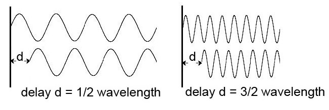
Phasing has been discussed in other
modules as well, for both the acoustic environmental
situation, and the electroacoustic
processing that simulates that phenomenon. Here we will
simply note that when a reflected sound combines with the
direct signal, there is constructive and destructive
interference patterns created where specific frequencies will
cancel, depending on the delay in the reflected sound,
namely those frequencies that are out of phase by a
half wavelength, as shown here at the left, for both the 1/2
and 3/2 wavelengths that are harmonically related as the 1st
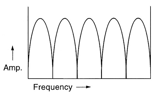
and 3rd harmonics. The frequency response of phasing on the
spectrum in a series of narrow notches called a comb
filter, shown at the right.
In this case, it is the narrow notches in the spectrum caused
by phasing that are most noticeable, particularly in a moving
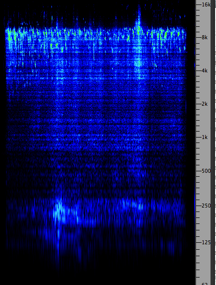
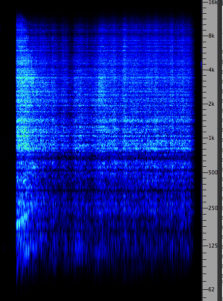
broadband spectrum, as shown in this video.
|
Frequency
response of phasing |
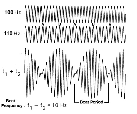
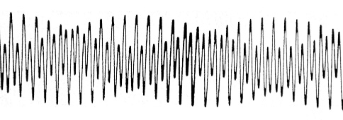
Beats are created when two frequencies
combine that are close apart, usually less than 10 Hz. Again,
it is a process of constructive and destructive interference
that is involved. In this diagram, two frequencies 10 Hz
apart, when combined, show points of destructive interference
marked A, and points of constructive interference marked B,
corresponding to out of phase and in phase,
respectively. The beat frequency (10 Hz in this case)
is the exact difference between the two frequencies.
First-order beats
between two tones, 10 Hz apart, showing their summation
and amplitude
modulation pattern
The result is heard as a periodic rise and fall in terms of loudness
changes, and the waveform can be described as a form of amplitude
modulation. These are called first-order beats,
and are frequently used by musicians when adjusting, for
instance, multiple strings that need to be in tune with each
other.
The accuracy of this is quite striking, because the
closer the strings are to being in unison, the slower
the beats become and the easier it is to hear the effect of
the difference. When heard as separate pitches, despite our
sensitivity to pitch, that difference is unlikely to be heard.
Beats
between 100 and 110 Hz where the difference is
gradually reduced
|
Beats
between 1000 and 1004 Hz, heard separately and
together (Source: IPO 32)
|
However, the
pitch ascribed to the fused tone with beats is the average
of the pitches of the two component tones. In the following
example we hear the combination of 200 Hz and a tone that is
1/4 semitone higher, beating together. Then we take out the
lower tone, and the pitch rises; then we take out the lower
tone, and the pitch falls, showing that when combined, the
brain averages the two tones in terms of pitch.
Beat
combination, with each component omitted in turn.
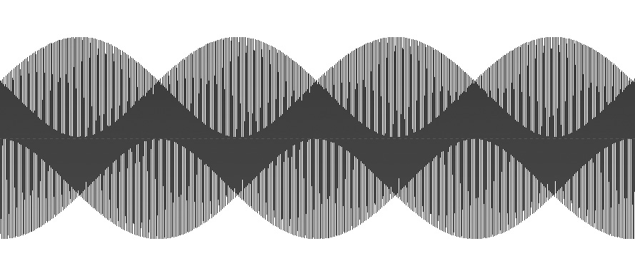
Second-order beats are also very
interesting, and produce a much more subtle form of
modulation, not in amplitude, but in the phase
relationships involved. The mistuning, in this case, is
between harmonics, such as his mistuned octave,
fifth or fourth intervals, and there this phenomenon plays
an important role in pitched based music involving intervals
and chords. Let’s hear the effect with just sine tones
first.
Beats between 100 and 201 Hz
|
Beats between the octave, fifth
and fourth, keeping the difference at 4 Hz
(Source: IPO 32)
|
You can hear some form of pulsation going on here,
but it is not a change on amplitude, and therefore loudness,
as is the case of first-order beats. These two diagrams show
the waveform involved in the 100 + 201 Hz example, where you
can verify there is no change in overall amplitude, but
rather a constantly changing waveform.
Second-order beats between a mistuned octave
The explanation involves a constantly
changing phase shift, as shown in the following diagrams.
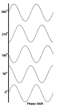
|
The
phase shift between 100 Hz combined with 200 Hz
frozen at various phase differences
|
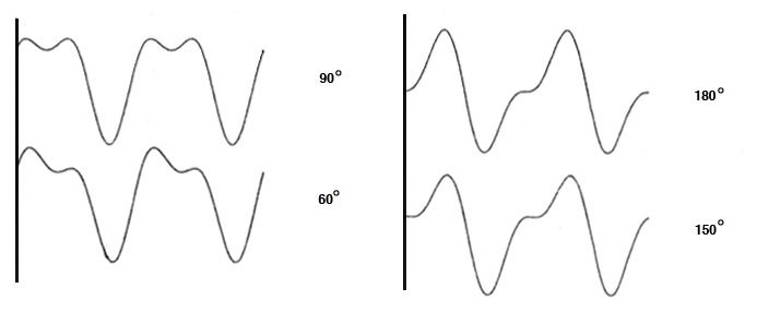
At the left, starting at the bottom, we see the phase
shift in a sine wave for 1/4, 1/2, 3/4 and a full period
or wavelength, identified in degrees, namely 0°, 90°, 180°,
270°, and 360° at which point it returns to be the same as 0°.
At the right, we combine the 1st and 2nd harmonics with
different phases between the two signals. The
second-order beats we saw and heard above create a similar
situation with the mistuning by 1 Hz – the phase relationship
between the two signals is constantly changing as you can see
by examining the left-hand waveform above more closely.
The ear is sometimes referred to as being insensitive
to phase differences (as we discussed in Fourier analysis
where the phase component was ignored), but that is not true
when the phase difference is constantly changing, as
shown here. In fact, secondary beats are a result of
auditory processing in the brain.
An intriguing variation of secondary beats
occurs when the mistuned frequencies are presented dichotically
to the brain, that is, where one tone is presented to the left
ear and the other to the right ear on headphones.
These are also known as binaural beats and are known to
have enthusiasts who listen to them for long periods of time
in order to affect their brain waves.
The principle is entrainment, that is, synching up
brain waves (such as alpha rhythms around 8-12 Hz) to the
beating pattern. Other listeners interpret the constantly
shifting phase differences as interaural time delays
(ITD) as we documented in binaural
hearing. The impression is that the sound is rotating
inside your head! You decide.
Binaural
beats between 200 and 401 Hz, presented dichotically
Index
B. Masking and Critical Bandwidth. Now
that we have covered how sound waves combine, and the
special cases where the combination, one might say, is
greater than the sum of its parts, we turn to the
psychoacoustic processes that allow us to separate
the incoming cumulative sound wave back into its components
– or not.
The familiar experience of noticing that a loud sound
“covers up” or “drowns out” other sounds is more accurately
referred to in Psychoacoustics as masking,
with the louder sound being the masker. The level of masking
can be determined in a lab as the amount of increase
in the masked signal required to restore it to audibility.
This level is called the masking threshold.
It is important to remember that masking is a psychoacoustic
process that depends on the analysis of sound in the inner
ear. Other forms of signal reduction such as attenuation,
damping, absorption, interference, etc. are physical
acoustic processes of reducing sound energy. Masking is all
about audibility, and hence the domain of psychoacoustics.
While the sense that the masker is louder (and must be) to
mask another sound, what is less well known by the general
public is that the masker must also occupy the same
frequency range as the masked signal. That specific
frequency range is what is called the critical
bandwidth, a measure that was introduced in the
Vibration module as a
crucial aspect of spectral analysis. Before we demonstrate
this fact, let’s listen to two recordings, the first where
masking does not happen (birds and traffic), and
one where at least partially, the broadband sound of a
fountain masks traffic as the recordist approaches it.
Birds
and bridge traffic
Source: WSP Van 72 take 3
|
Click
to enlarge
|
Approaching
a fountain with traffic in the background
|
|
The birds, in this case starlings which are
quite loud, occupy a much higher frequency range than most of
the energy of the traffic, so in the language of the Acoustic Niche Hypothesis, they have their own
frequency niche. In the case of a closer match of
spectra, such as the fountain and traffic, it is difficult in
a recording to show “what’s not there”, or at least not
audible, but as the recordist approaches the fountain, the
traffic does seem less audible.
This effect has often been argued for the role of fountains in
urban sound design, but this brief example shows how tricky
this can be, particularly in terms of low frequencies
which are not significant with the fountain. In indoor
situations, low levels of white noise started being
included in open-office designs back in the 1970s, and in
fact, as we will see shortly, the broadband range of white
noise does have this masking capability. However, sounds with
sharp attacks, such as phones ringing, will still be audible
above or “through” the ambient noise. In fact, all signals are
designed for their optimum audibility, so masking is not an
easy solution.
17. Personal
Listening Experiment. On a soundwalk, try to
find examples of masking, either by approaching a constant
sound source, or one that is intermittent and will allow you
to compare the soundscape with and without its contribution.
For sounds that you can still hear in the presence of the
masker, what qualities do they have, and conversely, if they
are masked, why was that?
You might not expect to find a masking example in symphonic
music, but they are plentiful in the works of the American
composer Charles Ives. One notable example, which suggests
that he must have been inspired by his soundscape
experience, is Central Park in the Dark, composed in
1906. There is a sequence (around 5') where the sounds of a
jazzy nightclub build into a crescendo and suddenly stop,
revealing the ambience created by the string section which
according to the score, has been there all the time.
Here is an experiment with different
sized bands of white noise designed to mask a 2 kHz tone heard
in 10 steps. There are five sequences: (1) the tone by itself;
(2) the tone masked by broadband noise; (3) the tone masked by
a bandwidth of 1000 Hz; (4) the tone masked by a bandwidth of
250 Hz; (5) the tone masked by 10 Hz. Count the number of
steps you can hear, and does it change as the bandwidth
narrows?
|
2 kHz masked by noise in
decreasing bandwidths
Source: IPO 2
|
Click to enlarge
|
The choice
of 250 Hz in this example is because at 2 kHz, the critical
bandwidth is about 250 Hz. This means that this very
narrow bandwidth (1/8 of the centre frequency) is sufficient
to result in masking. Therefore you likely heard the same
amount of masking in the broadband noise, the 1000 Hz
bandwidth and the 250 Hz bandwidth (probably 4-5 steps in each
case), but not with the 10 Hz final example.
This result also assumes relatively normal hearing sensitivity
at that frequency, and it also means that the group of hair
cells in that region along the basilar membrane are all
reacting to the same stimulus (tone plus noise) and
cannot distinguish the signal in the midst of the noise. In
fact, this is a standard method for measuring critical
bandwidth.
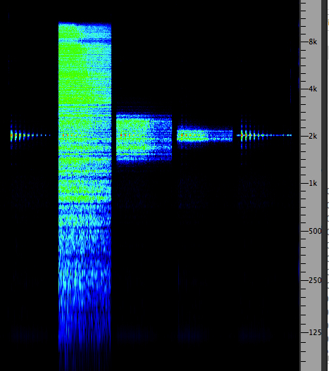
Here is a set of diagrams showing how broad
the range of frequencies is that are affected by masking for
two specific frequencies, and white noise.
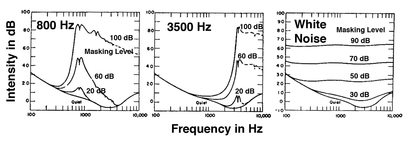
Masking levels for two frequencies and white noise
The first two diagrams show the masking capability of two
frequencies, 800 Hz and 3.5 kHz at three different levels
(loud, medium and quiet). However, in all cases the bandwidth
is not symmetrical – there is a tendency to mask
higher frequencies more than lower frequencies, shown as
a gentler slope above the centre frequency. However, with
broadband white noise, masking levels are evenly distributed
across the audible spectrum.
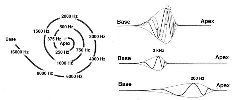
The reason for the so-called upward masking goes back
to the physiology of the inner ear, where we learned that high
frequencies are analyzed at the entrance to the cochlea along
the basilar membrane, referred to as the base in these
diagrams.
If masking interests you further, you can try three separate experiments here
to experience upward masking and what is known as
forward and backward masking. Forward masking refers
to the masking of a tone by a sound that ends a short
time (up to 20—30 ms) before the tone begins, which suggests
that recently stimulated hair cells are not as sensitive as
fully rested ones. Backward masking refers to the
masking of a tone that begins a few milliseconds later
(up to 10 ms). Backward masking apparently occurs at higher
centres of processing where the later arriving stimulus of
greater intensity overtakes and interferes with the weaker
stimulus.
Critical Bandwidth. At this point,
we have identified two important roles for the critical
bandwidth, which can be thought of as the resolving power
of the ear for simultaneous frequencies in a spectrum.
This means that timbre perception includes a spectral
envelope of resonance regions along the basilar membrane
based on hair cells firing that are a critical bandwidth
apart. This spatial representation of spectrum analysis is
projected onto the auditory cortex as a spatial pattern.
Secondly, we have just demonstrated the role that critical
bandwidth plays in masking. Sounds whose spectra are
more than a critical band apart will not mask each other, no
matter how loud, whereas those that partially overlap will
show some degree of masking, and those that overlap completely
(such as with a broadband noise) will show a high degree of
masking. In other words, the masking sound is stimulating the
same group of hair cells more strongly than the sound
being masked.
A third role involving the critical bandwidth introduces a
somewhat surprising connection between the psychoacoustics of
critical bandwidth and the impression of consonance.
This was at first surprising because the term consonance had
been associated for centuries with musical intervals.
Moreover, what was considered consonant in Western musical
practice (or its opposite, dissonant) had changed over time
and therefore seemed to be culturally determined.
As with most classical psychoacoustics, the
tests start with sine tones as opposed to the type of complex
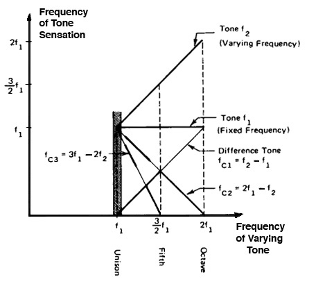
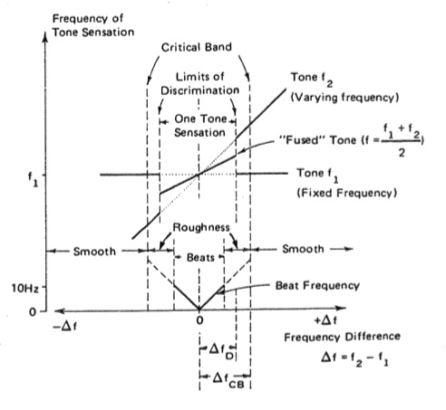
spectra found in musical timbres. Here is a basic
demonstration where two tones pull apart in frequency, and we
hear the following effects as diagrammed below where f1
is a constant tone, and f2 rises upwards from a
unison. There are three distinct (but overlapping)
impressions, as shown in the left-hand diagram:
- the region of one-tone sensation, first with a beating
pattern that represents the small difference in the two
frequencies, and whose pitch is the average of the two
frequencies (as shown by the skewed line in the middle and
beat frequency in the region below 10 Hz)
- the
beats become increasingly rougher past about 10 Hz,
and the threshold is crossed into a two-tone sensation,
referred to on the diagram as the “limits of (frequency)
discrimination” ΔfD meaning two tones can be
perceived
- the
roughness disappears at the frequency difference
equal to the critical bandwidth ΔfCB, and
the two tones appear to be in a smooth, consonant
relationship, as at the end of the following sound example
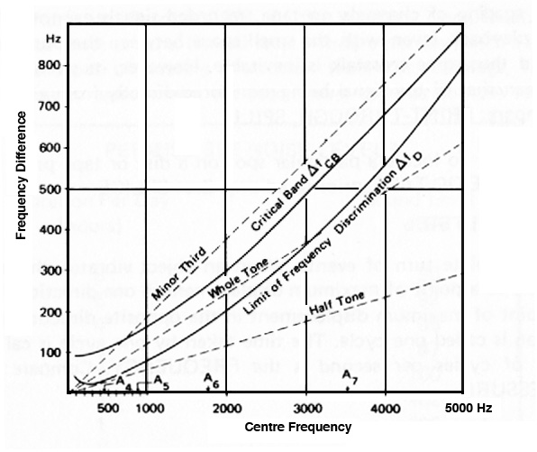
Frequency discrimination between two tones (left) and critical
bandwidth and frequency discrimination (right) correlated to
frequency range
Two sine
waves, one fixed at 400 Hz, the other ascending from 400 Hz
to 510 Hz at which point it is separated from the first by a
critical bandwidth
The
right-hand diagram above shows how the critical band
ΔfCB and the limit of frequency discrimination
ΔfD are related (the former being larger) in
relation to some common musical intervals. Above 1 kHz, the
critical band is a bit less than 1/4 octave, the minor third,
and therefore the 1/3 octave spectrogram tends to represent
mid to high frequencies the way the auditory system does, and
certainly better than the FFT. Below 400 Hz, the critical band
stays about constant at 100 Hz. The complete set of values is
tabulated in the Handbook Appendix E.
Personal
haptic experiment. Get the help of a
friend (preferably with a very steady hand) and two very
sharp pencils (but not anything similar that could
puncture the skin). Have your friend practice holding the
two pencils together at different distances apart,
including very close together (a fraction of an inch or
centimetre). You are going to close your eyes, and your
friend is going to lightly touch you with the two points.
It is your job to say whether you are feeling one point or
two. We suggest you start with your arm, as the points
will probably have to be quite far apart before you can
get a two-point sensation.
Once you’ve found that distance, have your friend touch
various parts of your hand with the points very close
together. You can alternate using one or both points, but
what will be interesting is how close the points can be
for you to get a two-point sensation in that location. You
can see the experimental results below for all parts of
the body, which show that the hands, face and feet are the
most sensitive places for this kind of touch
discrimination. We’ll leave it to you and your friend as
to whether further exploration is advisable.
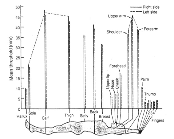
Limits of two-point touch discrimination on various parts of
the body
In summary, the relationship between
critical bandwidth and consonance can be summarized in the
following diagram where maximum dissonance (or
roughness) between two tones occurs at 1/4 critical
bandwidth, and maximum consonance occurs at a
critical bandwidth. The sense of roughness and
dissonance is the result of the same group of hair cells
responding to the two tones, whereas consonance in this
psychoacoustic sense, means that different groups of hair
cells are firing independently and not “interfering” with
each other.

Critical bandwidth correlated with consonance and dissonance
Plomp and Levelt calculated these values
assuming six harmonics in each tone, with the
result, shown here based on 250 Hz (approximately middle C),
that the intervals
typically regarded as consonant in Western music scored
highest in terms of this measure of psychoacoustic
consonance.
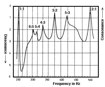
Consonance prediction for various intervals based on critical
bandwidth
The unison
(1:1) and the octave (2:1) have matching harmonics, so by
definition, they are the most consonant. The interval of the
5th (3:2) scores next highest, then the major 6th (5:3),
perfect 4th (4:3), and the minor and major thirds (6:5 and 5:4
respectively). There might well be disagreement about the
exact ranking of these intervals, particularly the thirds and
sixths, but the overall pattern seemed to confirm Western
practice, despite the reference to Just
intonation rather than Equal
Temperament.
At first glance, it might seem that this
suggests a “universal” justification for Western music
practice – a highly suspect claim – so it is worth noting that
what this psychoacoustic evidence actually confirmed was more
along the lines that timbre affects tuning. In fact,
we got a sense of that in the Vibration module experiment where
exact octave relationships between sine tones sounded flat,
indicating that an enriched musical spectrum influenced pitch
judgements.
As a final, suggestive example, we can refer to Indonesian
tuning systems (slendro and pelog) which are based on bronze
instruments with decidedly inharmonic spectra, and are
largely tuned by ear during their production and hence are
widely variable in different gamelan orchestras. Although this
music has been imitated on Western musical instruments with
pitch approximations to the tempered 12-tone scale, something
seems to have been lost.
Index
C. Non-linear Combination. Auditory
processing, like electroacoustic processing, is not always
linear. Note that we are not referring to linear as opposed
to logarithmic as applied to a specific parameter
such as frequency. In fact, in the inner ear, frequency is
processed on a logarithmic scale, where octaves, for
instance, are equally spaced, and therefore the coloured
spectrograms we use here are also on a log scale.
In this context, think of non-linear as non-proportional,
in the sense that the output is not a scaled version
of the input. Rather, the output includes elements such as
frequencies that are not present in the input, similar to
electroacoustic modulation.
In this section we will summarize some of the well-known
aspects of auditory processing that seem to add tones to the
perceived input, known as combination
tones. They are examples of distortion
in a signal, such as over-driving a loudspeaker and hearing
a distorted version of a sound. Similarly, combination tones
depend on the intensity of the sound you are
listening to, and will likely disappear at lower levels. As
such, some people find them annoying to listen to, so you
are welcome to reduce their volume in the examples. Also,
they are hard to localize in space, and are more likely to
seem like they are coming from inside your head.
We will start with one of the more obvious combination
tones, namely the difference
tone. In this example we hear 1500 Hz combined
with 2000 Hz at a fairly strong intensity level, and it’s
likely you will hear a buzzy lower tone corresponding to the
frequency difference, namely 500 Hz. You might have heard
something similar in a blown whistle, such as one used by a
sports referee or police officer, at least in times past.
These whistles often had two sections that each produced a
different pitch.
Combination
of 1500 and 2000 Hz, producing a 500 Hz difference tone,
heard alone at the end
Combination tones heard between a constant
tone f1
and a rising one f2
The
above diagram and the sound example below demonstrate that
there may be multiple combination tones heard (at
sufficient loudness), in this case produced by a constant
tone f1 combined with a similar tone f2
that rises an octave above the first one. The difference
tone can also be heard rising, but if you hear one
or more descending tones, they are combination
tones at frequencies 2y - x and 3y - 2x, all caused by
distortions in processing in the inner ear.
As you can see in the spectrogram, they do not exist in
the signal itself (where no descending lines occur in the
spectrogram) although some other artifacts may be seen
there, probably caused by the electronic circuit itself
which may exhibit non-linearities as well. The summation
tone (x + y) is seldom heard.
A 500 Hz constant tone combined
with an ascending tone, from 500 to 1000 Hz
producing various combination tones
|
|
These
final two examples cleverly reveal the presence of
combinations tones without playing the example very
loudly. In the left-hand example, the tones are 1000 and
1200 Hz, hence producing a difference tone (2y - x) of
800 Hz. Next a so-called probe tone at 804 Hz is
added and this produces a beating sensation with the
difference tone, heard inside the head.
In the right-hand example, similar to the one above, the
upper tone rises from 1200 to 1600 Hz and some other
combination tones can be heard.
1000 and 1200 Hz with a probe
tone of 804 Hz (source: IPO 34)
|
The upper tone rises from 1200
to 1600 Hz producing changing combination
tones (source: IPO 34)
|
Index
D. Auditory fusion and streaming.
At the level of auditory processing in the brain,
one of its key tasks is to identify incoming
patterns as belonging to the same sound source, and
not to other possible sources. In the previous
module, we showed how precedence effect
favoured what arrives first and presumably loudest,
with later arriving signals being momentarily
suppressed. Similarly, cocktail party
effect described our ability to focus
on one stream of sound coming from the same
direction. On the other hand, in this module, we
have shown how sounds occupying a similar frequency
range can mask another quieter sound,
including those a few milliseconds before or after.
When an incoming stream of acoustic information
produces a singular percept (a term that
indicates not just a “response” but a complete
perceptual image), we can say that auditory
fusion has been achieved. Musical tones
comprised of harmonics fuse together easily because
of the common periodicity involved, to which
pitch is ascribed. Inharmonic sounds, such as those
found in bells and metallic sounds, lack this
periodicity but still can fuse based on other cues,
and be assigned a somewhat arbitrary pitch.
Vocal sound perception, as described in the next
module, has the multiple task of identifying a voice
(probably based on similar cues for auditory
fusion), rapidly detecting a stream of (hopefully)
familiar vowel and consonant patterns, and detecting
the larger scale patterns of paralanguage
(i.e. non-verbal cues) that will also be discussed
in the next module.
For more general types of sounds,
both musical and environmental, here are some other
cues that aid auditory fusion, besides a
common direction. The first is onset synchrony.
If all of the spectral information begins together,
or within a short interval, then the brain will
likely recognize it as coming from a single source.
In the following synthesized example, you can hear a
sharp, unambiguous attack in the first sound, then
two elongations of the attack (up to 100 ms), which
then separate into short repeated attacks. Of course
if these become very dense and inseparable, then a
texture will be identified. Contextual
learning will likely assist in distinguishing
between two events coming from two sources in the
same direction, or one composite sound event with
component elements, such as a machine sound.
Onset synchrony leading to a
separation of elements
Many of the perceptual grouping
principles we are going to encounter in the rest of
this module are related to Gestalt perception,
an approach that was common in psychophysics in the
1920s and 1930s, but predominantly restricted to
visual examples. At that time, there was little
methodology available for analogous work with aural
perception as there is now, so it is not surprising
that Gestalt principles are once again being called
upon for auditory perception.
One of these principles is called common fate.
Elements that share a common characteristic are more
likely grouped together into a singular percept. In
musical ensembles, the aim is usually to blend
similar voices or instrument groups together, such
as positioning the performers close together,
rehearsing synchronous attacks, maintaining the same
pitch tuning, and balancing loudness levels. These
elements guarantee blend and fusion, and also
enhance the overall volume and timbre, referred to
as choral
effect. Micro variations, within
perceptual and performance limits, apply, but the
global effect is an enriched sonic grouping, unlike
amplification of a single instrument or voice, which
will lack the same internal dynamics in the overall
sound.
In this example, based on John Chowning’s work at
Stanford in vocal synthesis, we hear three examples
of a fused spectral complex, each beginning on a
single pitch, then with other spectral elements
added, out of which a female singing voice
miraculously appears. Why?
Because the vocal formants in the singer’s voice
suddenly have the same synchronous vibrato.
Therefore, by common fate, we readily identify one
singer, not a chord or timbre. In the fourth and
last instance, the three pitches combine into a
chord, all spectral elements are added, and then
three independent rates of vibrato are
added to each voice and we have a sung chord with
three singers.
Synchronous vibrato with a
singer
Source: Cook exs. 73-76
|
Click to enlarge
|
Although this next example would
not count as auditory fusion, we might refer to it
as “soundscape fusion” in that it mixes together
several separate elements recorded at separate
times in Vancouver harbour, into a plausible
soundscape portrait of that environment. A
listener recognizes the semantic appropriateness
of a boat horn, waves, seaplane, and a Vancouver
soundmark called the O Canada horn. Of course a
local resident will know that the O Canada horn
sounds at noon, so if we combined it with the Nine
o'clock gun, which sounds every evening, the
listener might recognize the inconsistency and
question the veracity of the recording. Others
might not.
Vancouver harbour
mix
Soundscape Vancouver,
CSR-2CD 9701
|
Click to enlarge
|
On the other hand, listeners familiar with media
productions often ignore blatant aural
inconsistencies. An actor may well have been
studio recorded and the voice exhibit boomy room
resonances, and yet the scene being projected is
clearly outdoors.
Auditory
streaming. Once a specific sound can be
identified as percept, it can be grouped
together with similar sounds that flow into what
psychoacousticians call an auditory stream.
Again, certain gestalt principles seem to apply.
One has to do with occlusion, which is
usually illustrated with a visual example. The
following messy visual display seems to make no
sense until we can identify an occluding object
in front of it (as with the link).

A pattern that only makes sense when we see
the occluding object here.
Something similar can happen when
an auditory stream is momentarily masked
by another intermittent sound. We assume (not
just logically, but perceptually) that the
masked sound continues its trajectory “behind”
the masking element. In this example, we hear
an up and down glissando with gaps that are
then filled in with noise, and suddenly the
gaps in the glissando disappear. This is
followed by a violin with similar gaps that
are filled in with noise.
A glissando and
a violin with gaps filled in with
noise bursts (source: Cook
5)
|
Of course in the acoustic world,
an occluding object, even a building, does
not prevent some frequencies (usually the
lower ones) from diffracting
around it, so this aural version works best
with intermittent masking sounds which don’t
appear to disrupt the ongoing auditory
stream percept.
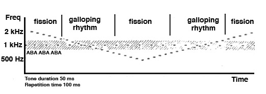
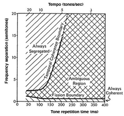
Two of the main
parameters for auditory stream formation
with pitched tones is the tempo of
the tones (the number of tones per second),
and the frequency distance between
successive tones. The left-hand diagram
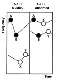
shows that if the frequency separation is
fairly large, tones A & B will group
because of their proximity, as will
X & Y. However, when the frequency
difference is less, then A will group with
X, and B with Y in two streams.
Tone
grouping based on proximity (left), and
tone segregation dependency on
frequency distance and tempo (right)
The right-hand diagram shows that as the
frequency difference gets larger, tones
are always segregated, that is,
they do not form groups, a condition also
referred to as fission. Similarly,
tones that are only a semitone apart, like
a trill, are always coherent at
any tempo. In between is an ambiguous
range where your own perception
determines whether the sequence is
coherently streamed.
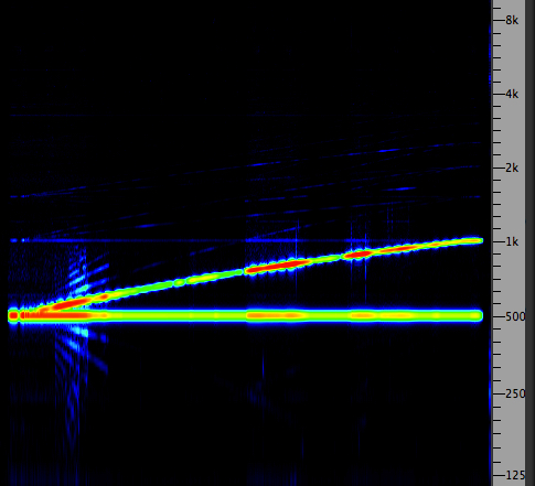
The following is a classic example by Leon
van Noorden, where a repeated sequence of
ABA tones at a fast tempo (10 tones/sec)
start an octave apart and then the higher
tone descends. The sequence first shows
segregation (i.e. fission), where you can
pay attention to the high descending tones
or to the steady low tones. But
then, as they approach each other, a
“galloping” rhythm groups the tones
together in rhythmic triads.
It is interesting to try to hold onto that
grouping as the descending tones get
farther apart again – but inevitably you
have to give way to fission in the
pattern. Likewise, when the tones start
ascending again. Have some fun with this
example.
|
Tone
sequence progressing from
fission to coherent streams
and back
Source: IPO19
|
A subtler
example combines auditory fusion with
coherence. A sine tone A alternates with
a complex tone C based on a fundamental
of 200 Hz. When tone A does not
correspond to one of the harmonics of
the complex tone, it is segregated out
and has its own slower repetition tempo.
But as it ascends, it comes into tune
with the 2nd and 3rd harmonics of the
complex tone, and if you listen
carefully at these points, you can hear
the tempo of tone A double as it
streams with those harmonics.
This is an interesting case that sheds
some light on the larger question of
whether any tone is heard as a pitch
or part of a timbre. The
surprising thing here is that the tone
can be a harmonic and be heard apart
from the typical fused harmonic
spectrum.

|
A sine
tone alternates with a
complex tone and streams
with a harmonic when it
matches its pitch
Source: van Noorden
Spectrogram
|
Another
fun demo of pitch streaming based on proximity
is when two common melodies are
interleaved, that is, their notes
alternate. If they are initially in
the same range, nothing can be
identified, but as the second melody
is transposed higher and higher, bits
of each melody start appearing until
the separation is complete, and you
can listen to whichever melody you
like.
Two
interleaved melodies that
separate
Source:
van Noorden
|
|
In the music for
solo instruments in the Baroque
period, it was customary to imply
two or more different melodies at
the same time, as long as they were
sufficiently separated in pitch.
Usually this intention was not
indicated in the score, as in this
simple Minuet from Bach’s Partita
No. 1 where in fact all of the
notes are articulated as having
equal value in the score. However,
by sustaining or articulating
particular notes differently, they
will stream into their own melody,
as indicated above the score for the
right-hand opening melody.
Bach Minuet
from Partita No. 1
|
|
This kind of
streaming can be heard in various
types of African drumming,
particularly those from Ghana,
which has so-called
interlocking parts on
different drums and percussive
instruments. Each part is
relatively simple, but together
they form a rhythmic complexity
where you can listen to the
overall pattern, or just a
component.
This type of music inspired Steve
Reich in his early work, such as Drumming
(1970-71) which, despite being
labelled as minimalism, actually
developed an internal
complexity which allowed
listeners the freedom to listen to
internal patterns that could be
heard as separate and evolving
streams.
Index
E. Cognitive
processing and hemispheric
specialization. The
structure of the brain and its
neurological functioning is
beyond our scope, but we can
outline some basic features
that help us to understand how
sensory information is
processed there.
It has long been known that
different areas of brain have
their own specializations, and
that injury (e.g. lesions) to
one part may show an
impairment of specific
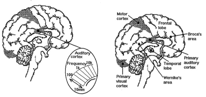
functions. This diagram shows
the location of some important
areas, including the Auditory
Cortex, with a reminder
that the spatial map of the
frequency analysis of incoming
signals, as performed by the
hair cells in the inner ear,
is projected onto the auditory
cortex with that spatial
display intact.
We also know that multiple
areas of the brain are
stimulated by incoming
auditory stimulation, even
during sleep. The following
PET scan shows activity in at
least two areas, the auditory
cortex and the frontal lobe
which controls executive
functions such as attention
and motor functions. In this
case, the brain is responding
to tones while in a deep state
of sleep.
We know the anecdotes about a
mother being wakened to her
baby’s cry, or some similarly
salient sound, and here is the
modern understanding of that
phenomenon. If this can happen
during sleep, then it’s clear
that more complex
communication between visual,
linguistic and other areas of
the brain will reflect normal
functioning during waking
consciousness.
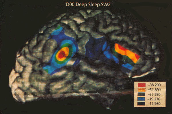 PET
scan of the brain during
sleep in response to tones
PET
scan of the brain during
sleep in response to tones
One of the
most intriguing aspects of
brain behaviour is the role of
the two hemispheres,
left and right, joined by a
massive set of fibres known as
the corpus callosum,
shown in the visual diagram
below, that allows the
hemispheres to communicate
with each other.
Most motor and sensory input
is processed in what is called
a contralateral mode;
for instance, the left hand is
controlled by the right
hemisphere, and the right hand
by the left hemisphere. Visual
information is processed that
way as well, keeping in mind
that both sides of the visual
field, left and right, go to
both hemispheres, after being
reversed in the eye itself.
Smell is one of the few
ipsilateral modalities,
that is, the left and right
nostrils, respectively, are
connected to the same
hemispheres.

Contralateral
control of the hands
|
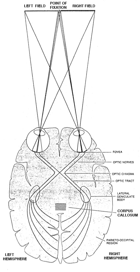
Click to enlarge
|
Examples of
contralateral brain control
mechanisms for handedness
and vision
It is important to remember,
however, that auditory
information from both
ears goes to both
hemispheres as well, but
only with what is generally
estimated as a 60/40 split
contralaterally. In
other words, there is a small
preference given to the
hemispheres for auditory input
from the opposite ear.
Hemispheric
specialization (or
cerebral dominance) refers to
particular processes that each
hemisphere specializes in,
although it should be kept in
mind that either hemisphere
can learn any of these tasks.
In general, the left
hemisphere is involved with language
and logical functions,
particularly for right-handed
subjects, keeping it mind that
handedness is contralateral.
In left-handed subjects,
however, language functions
seem equally divided between
either left or right
hemispheres. Broca’s area is
associated with speech
production, and Wernicke’s
area with speech
comprehension, and these are
usually found in the left
hemisphere. As a result, the
left hemisphere has often been
referred to as “dominant”, but
that designation can be
misleading.
The right hemisphere, in
contrast, specializes in visual,
spatial and holistic
analysis, and has been
mistaken for handling musical
activities. This misconception
arose in the 1960s and 1970s
when studies with musically
untrained subjects showed a
left-ear preference for
music recognition tasks when
presented dichotically (i.e.
separate signals going to each
ear via headphones). What was
more likely happening was that
melodic patterns were being
listened to as a whole,
basically as shapes.
When more refined tests in the
1970s compared music students
with their musically untrained
counterparts, the music
students, trained to be
analytical about pitch and
intervals, showed a right-ear
preference. Interestingly
enough, when those tests were
carried out with music
professionals, it showed that
they could use either holistic
or analytical modes of
listening about equally, and
could probably readily switch
back and forth between them.
Therefore, simplistic notions
that language is “in” the left
hemisphere, and music “in” the
right (and where would that
leave environmental sounds?)
need to be abandoned in favour
of listening strategies that
are characteristic of each
hemisphere.
Diana
Deutsch, the British-American
psychologist working at the
University of California in
San Diego, became well known
for her studies in music
perception based on
hemispheric specialization. A
striking example is how simple
tone patterns heard dichotically
(i.e. fed separately to each
ear) are “re-arranged” in the
brain according to the Gestalt
principles we have illustrated
above.
Listening
Experiment.
Listen to this recording
of melodic tones on
headphones and describe
the melodic patterns you
hear. Does it sound like
pattern A (a descending
line in one ear and an
ascending one in the
other), or pattern B (a
mirrored down/up and
up/down in each ear)?
Tonal
pattern in each
ear
Source: Diana
Deutsch
|
|
The most common
percept is pattern
B, the down/up pattern in
one ear, and the up/down
pattern in the other. Two
crossing lines, pattern A,
is very difficult to
achieve without the sounds
involved being very
different, and so this
pattern has traditionally
been avoided in musical
counterpoint. In fact,
pattern B is not
the stimulus pattern at
all! Listen to this
example of the left ear
signal only, then the
right ear signal only.
Left
signal followed by
right signal
Deutsch described the
effect as the brain
‘re-organizing” the input
into a pattern consistent
with minimum proximity
between the notes. As you
heard, the actual “melody”
is very angular, jumping
between higher and lower
tones, so the auditory
system re-assigns
them to each ear in more
coherent step-wise
patterns.
In case you’re thinking
this is a modern invention
of digital synthesis, the
effect was used by Peter
Tchaikovsky in the last
movement of his Symphony
No. 6 in 1893. We
hear a descending line in
the violins, but in fact,
neither the first
or second violins play
that melody, as you can
see from the score below.
They play an angular
version of it where every
other note in the
descending line is
assigned to each group.
Instead of our dichotic
listening experiment with
the left and right ears,
the two violin groups in
Tchaikovsky’s day were
seated on opposite sides
of the stage.
 Tchaikovsky,
Symphony No. 6, 4th
movement theme
Tchaikovsky,
Symphony No. 6, 4th
movement theme
In this last example,
there is an element of
competing Gestalt
principles, so let’s
illustrate that in the
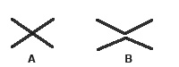
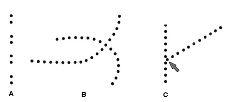
visual domain first. In
case A, do you see a
line of 8 dots, or 4
groups of 2? We readily
see 4 groups, because of
the principle of proximity,
just as with the melodic
tones. In case B, do you
see 4 lines coming
together or two lines
crossing. Again, the
latter because of what’s
called good
continuation. Now,
in case C, we test which
of those principles is
stronger when we try to
identify the dot being
pointed to. Is it part
of the vertical line or
the diagonal? Most
people would say the
latter, so the proximity
effect seems to be
weaker.
Again, headphones are
required. High and low
tones are heard
alternating. Once you
fixate on a particular
percept, switch the
headphones around.
Does the pattern change?
There is no right or
wrong answer, but check
out the commentary here.
Alternating
tones (source:
IPO 39)
F.
The acoustic community
and the Acoustic Niche
Hypothesis. Most
of the examples above
dealt with speech and
music, so we need to
turn our attention to
the larger context of
how sounds interact with
each other, which is at
the level of the soundscape
and bio-acoustic
habitats in
general. To do this, we
will follow the
emergence of these
concept in the work of
the World
Soundscape Project
(WSP) and
bio-acoustician Bernie
Krause in the
1970s, leading to the
present day.
An important step for
the WSP came with the
24-hour “Summer
Solstice” recordings in
June 1974, on the rural
grounds of Westminster
Abbey near Mission, BC,
where the birds and
frogs around a pond
formed an ecological
micro-environment. An
edited version of these
recordings consisting of
about 2 minutes per
original hour was
broadcast on CBC Radio
in stereo as part of the
radio series Soundscapes
of Canada in
October 1974, the other
programs being based on
the cross-Canada
recording tour the
previous year.
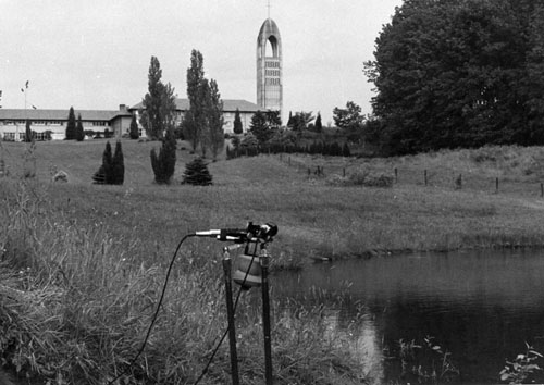
WSP
recording
setup at
Westminster
Abbey,
Mission, BC,
June 1974, on
the summer
solstice
|
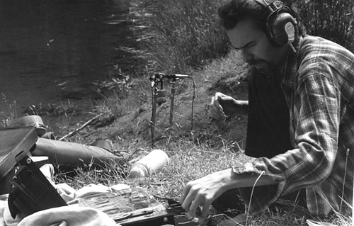
Bruce
Davis
recording with
the stereo
Nagra machine,
June 1974
|
The time compression for
each “hour” was
transparently achieved
with editing, with a
short verbal
announcement of the time
being the only
commentary. Therefore,
over the course of the
hour-long program, a
listener could
experience the
soundscape of an entire
day at this site,
something that would be
physically impossible
for an individual to do.
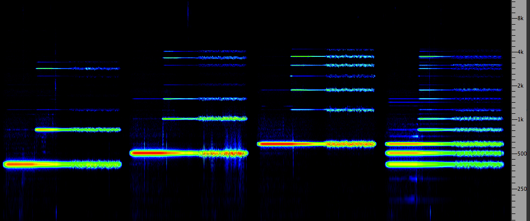
Solstice
recording 3 to
8 am
from
Program 5, Soundscapes
of Canada
|
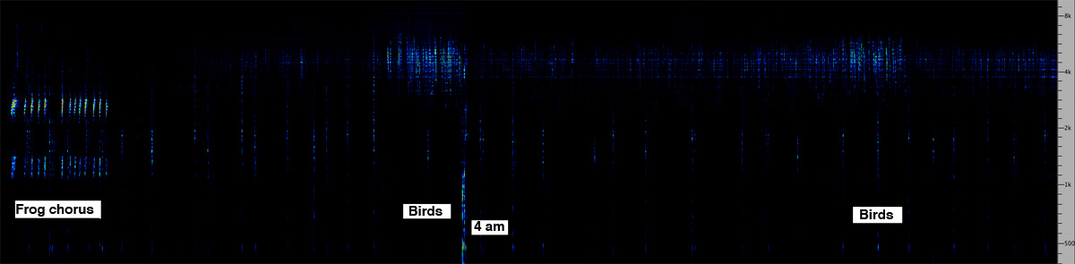
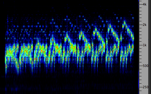
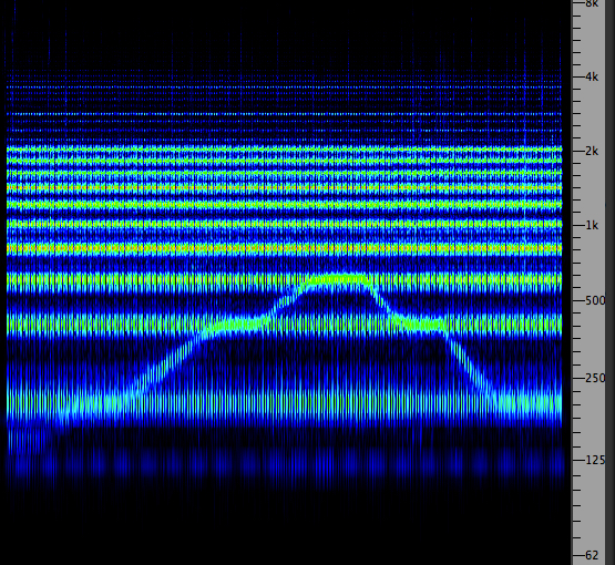
Spectrogram
of the period
just before
and after dawn
(3:30 am)
showing
frequency
niches for
frogs and
birds (click
to enlarge)
|
Even though the group
had little training in
bio-acoustics, the aural
“balance” of the
soundscape was
impressive. Species
soundmaking (mainly
birds during the day and
frogs at night) was
always dynamically
changing, but in such a
way that there was no
conflict in competing
sounds. The two key
moments at sunrise and
sunset involved dramatic
transitions from birds
to frogs and back again,
but their patterns
evolved naturally
without colliding. A
chart of the 24-hour
evolution of the
soundscape is shown
here.
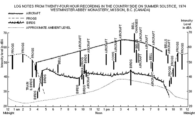 24-hour
log of sounds
heard during
the summer
solstice
recordings,
June 1974, by
the WSP
24-hour
log of sounds
heard during
the summer
solstice
recordings,
June 1974, by
the WSP
Having
just finished a study of
the Vancouver
soundscape, with its
typically chaotic noise
environments, it was
impressive to listen to
a soundscape that seemed
fully integrated and
functional. Most
importantly, it gave a
purpose to the field
tour in Europe the
following year which was
to find examples of
villages in five
different countries
where the soundscape of
a social and cultural
unit on the size of a
village could provide an
analogous, balanced
eco-system, one that
came to be modeled as an
acoustic community.
The result of the study
was the document Five
Village Soundscapes,
where very different
types of villages in
Sweden, Germany, Italy,
France and Scotland were
studied in 1975 as to
how sound played a
pervasive and positive
role in the life of the
community, even as they
were subject to
differing degrees of
modernization that might
challenge that
positivity.
The villages included a
modern manufacturing
village in southern
Sweden (Skruv, where a
glassworks, brewery and
two other industries
were located), a
traditional farming
village in Germany
(Bissingen, where a
textile factory was also
operating), a fishing
village in Brittany
(Lesconil), a mountain
village in northern
Italy (Cembra,
experiencing declining
population as people
migrated to the city),
and an academy town in
Scotland (Dollar, on
major highway and rail
routes, but with strong
links to the past).
From the sparse
Scandinavian village
soundscape, to the
French and Italian ones
centred on human
activity, and those
experiencing the effects
of industrial and
technological trends,
these villages presented
a range of examples
where sound still played
a largely positive
and pervasive role
in the definition and
experience of the
community. More detail
on this study, and the
Finnish update in 2000,
is available on the WSP
Database.
The WSP study drew
several conclusions
about the character of
the acoustic communities
they studied, some of
which were identifiable
within the language of
ecology. The first was
the variety of
sonic “species” that
were heard in these
villages. Instead of the
soundscape being
dominated by a few,
acoustically powerful
sounds, these
communities exhibited a
wide range of sounds
that could be heard on
soundwalks throughout
the village. The writers
noted that this
conclusion was rather
the opposite of the
cliché that life in the
modern city is “complex”
– culturally perhaps,
but not necessarily
aurally when a few
technological sounds
dominate.
The second
characteristic of the
acoustic community was
the complexity
of information gleaned
by the inhabitants from
everyday sounds. This
was often noted by the
researchers, but could
only be explained by the
inhabitants who had the
requisite knowledge of
context, culture and
history. Although the
experience of sound in
such a community is
shared, the
interpretations and
reactions of the
inhabitants can be quite
varied, depending on
personal experiences,
preferences, and their
relationships to the
community’s power
structures.
Finally, a third more
explanatory criterion
was identified, namely
how the variety of
sounds were maintained
in an ecological
balance. What kept
the variety (and
magnitude) of sounds
from overwhelming each
other and producing a
chaotic soundscape?
Acoustic communities,
when regarded on a macro
level according to the
WSP model, seem to have
evolved (as in the
examples described
above) according to
several balancing
factors related to
physical space, time
(e.g., rhythms and
cycles) and social
practice. In many cases,
economic, social and
cultural factors have
determined the physical
design and layout of a
village, town or city,
but each decision has an
acoustic impact, and so
it might be more
accurate to say that
there is a co-evolution
between acoustic and
cultural developments.
Clearly both aspects
need to be examined
together as part of what
we are calling an
ecological system.
During
this same period, an
electronic musician
named Bernie Krause
in California began
recording natural
soundscapes. Unlike
biologists who study
specific species, and
therefore try to record
their sounds
individually, Krause
recorded soundscapes as
a whole and became
fascinated with their
complexity. Once he was
able to perform a
spectrographic analysis
of these recordings in
the early 1980s, he
could confirm some of
his aural impressions
about that seemingly
organized complexity.
On a spectrogram where
frequency is on the
vertical axis, time on
the horizontal, and
higher amplitudes are
shown as darker lines,
he could see that
species’ soundmaking
fell into separate non-overlapping
frequency bands,
somewhat similar to how
the radio
spectrum is
divided into
simultaneous broadcast
frequencies.
This insight has come to
be called the Acoustic
Niche Hypothesis
(ANH), and is accepted
by landscape ecologists
as a key component model
of what can be called an
acoustic habitat.
It is clear that a well
functioning habitat
depends on acoustic
information that is
shared among different
species co-habiting the
eco-system. And, as with
all habitats, it is
potentially vulnerable
to change or threats to
its existence. These
threats in the form of
excessive noise that
blocks the acoustic
channel are also being
found in marine
soundscapes where sound
travels over very long
distances, including a
great deal of ship
traffic and other sound
sources that can disrupt
species communication on
which they depend.
More recently, the
Italian musician and
ecologist, David
Monacchi, has
systematically recorded
the soundscapes of
subtropical regions and
discovered further
evidence about the role
of the ANH in those
acoustically rich
habitats, as part of his
Fragments of
Extinction
project. He has
illustrated the spectra
of those habitats on a
real-time spectrogram
presentation, using the
SpectraFoo software,
similar to what we have
been using here (in fact
it was his use of
spectrograms that
inspired our own).
You can see and listen
to a variety of examples
by Krause and Monacchi here.
By applying this
approach to our
problematic urban
spaces, we can learn
from the bio-acoustic
examples, as well as
those we have
characterized as
acoustic communities,
that sound constitutes
an aural habitat, but to
be functional it needs
to operate on a human
scale, by which I
mean, populated by
sounds whose acoustic
properties are in a
similar range to those
we make as humans as
well as those of other
species. Here is a brief
example of an urban
development that seems
to have succeeded in
this regard.
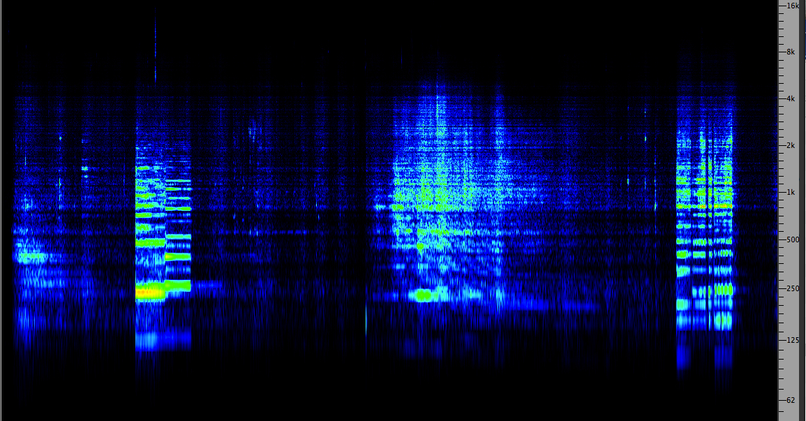
Granville
Island,
Vancouver
Source:
WSP VDat
5, take 17
|
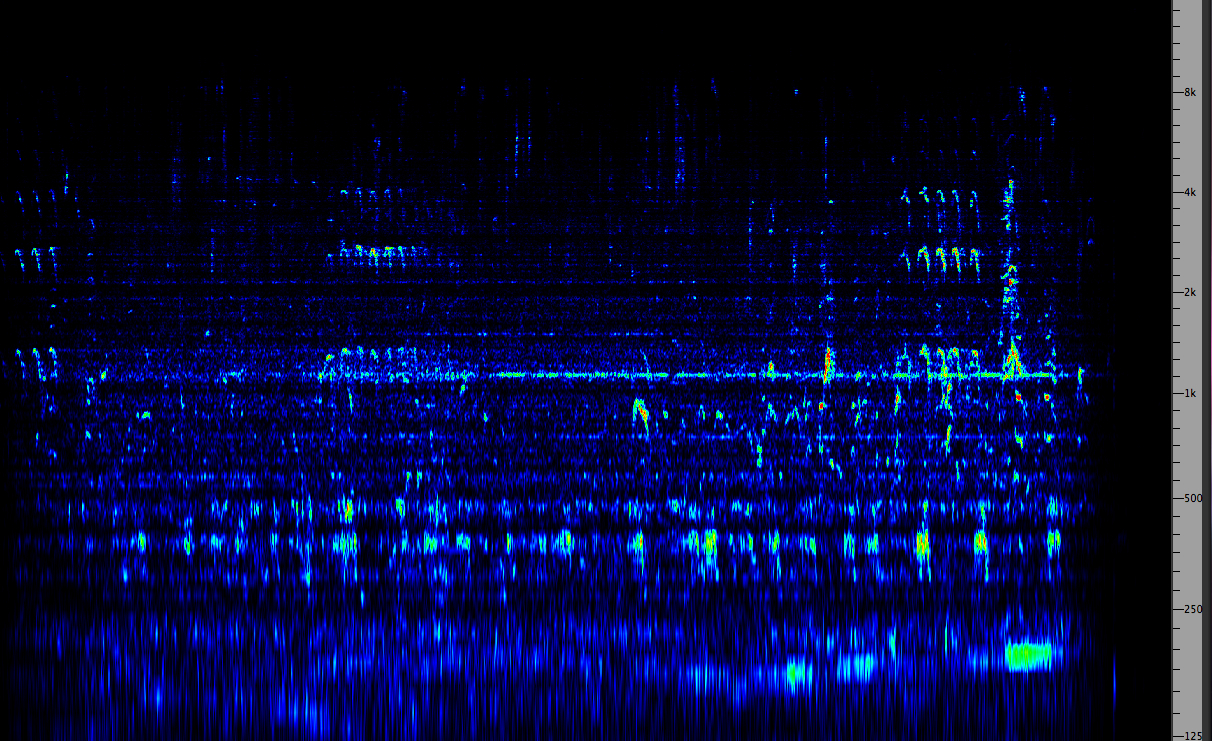
Granville
Island
spectrum
showing a
balance of
frequency
bands (click
to enlarge)
|
A balance in the
spectrum, loudness and
temporal behaviour of
all of the component
sounds is required to
make the system function
in a sustainable manner.
Of course, a certain
number of sounds and
events falling outside
that range (but within
safe limits) can be
accommodated within the
system without
jeopardizing it, and may
in fact be necessary if
they are expressions of
social cohesion. But the
aural pathways must be
kept open so that
listening can guide us.
Index
Q. Try
this review
quiz to test
your comprehension of
the above material,
and perhaps to clarify
some distinctions you
may have missed.
home

