 |
MICROSOUND |
Granular Synthesis and the Granulation of Sampled Sound
|
MICROSOUND |
The micro time level for sound, often referred to as microsound, is more properly termed the frequency-time domain which is a topic in engineering that applies to a wide range of contexts, of which sound is just one.
This domain can also be referred to as the quantum level of sound because we can speak of a particle of sound called a grain that is regarded as the smallest unit which constitutes sound, otherwise normally thought of as a wave.
The frequency-time domain is becoming increasingly important for sound and audio because the properties of treating sound at that level are the basis of many contemporary approaches to sound synthesis and processing.
We will cover these topics:
A) The frequency-time domain
B) Granular synthesis
C) Granulation of sampled sound
D) Studio demo's
Q) Review Quiz
home
A. The frequency-time domain. The traditional view of the time and frequency domains is that they operate independently, which is true at the macro level of the time domain. In that model, the time domain is regarded as starting at the waveform level (as in a sound editor or oscillator description), and the frequency domain is that of the spectrum, or “frequency content”, of a sound, as displayed in a number of conventional formats. In music, these domains correspond to rhythm and pitch, respectively, which can be combined in any melodic pattern.
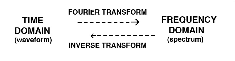
In acoustics and audio, one passes from the time domain of the waveform to the frequency domain of the spectrum via a transform, the most common of which is the Fourier Transform, and its more efficient version, the FFT (Fast Fourier Transform). Its process is to analyze the sound in terms of the strength or amplitude of a number of frequency bands extending over the entire frequency range. An inverse transform can then re-create the time domain signal as needed, as shown in this diagram.
We have already experienced this process with Convolution, in both the case of Impulse Reverberation where the signal is convolved with the Impulse Response (IR) of an acoustic space, and the special case of Auto-convolution where the sound is convolved with itself. The rule that was followed in each case is that:
convolution in the time domain is multiplication in frequency domain
This process means that each signal is analyzed in the frequency domain, and the respective strengths (amplitudes) of each frequency band are multiplied by each other and the result returned to the time domain by the inverse transform. Therefore convolution can be thought of as a time-frequency domain process.
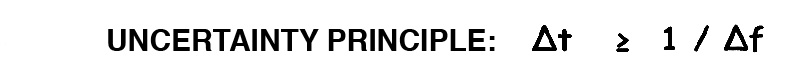
At the micro-level of the time domain (which is less than 50 ms), time and frequency are interdependent and linked by an Uncertainty Principle. This is the so-called quantum level of sound, by analogy to the quantum level of particle physics. The principle can be stated in general as shown here.
This principle is expressed in terms of a short window of time Δt compared to a “window” or band of frequency Δf. When we defined the basic properties of a periodic waveform we found that the period of vibration T was inversely proportional to the frequency f, such that T = 1/f, and so the uncertainty principle takes the same form by saying that a window of sound in time is inversely proportional to the frequency bandwidth. This means, the narrower the window of time, the broader the bandwidth, and vice versa. Therefore, to reduce the uncertainty in frequency (i.e. to narrow its bandwidth) you need a longer and longer time window.
You may be more familiar with the Heisenberg Uncertainty Principle which generally states that the position and speed of an electron at the quantum level cannot both be determined to the same degree of accuracy: the more you know about the speed of the electron, the less you know about its position. This makes sense because speed is the rate of change of position.
When we transition to the acoustic domain, the same principle applies because (as we learned in the first Vibration module) frequency is the rate of change of phase. A high frequency sound changes its phase rapidly, compared with a low frequency sound. Therefore for a given window of time, the bandwidth is inversely proportional. This can be verified fairly simply by cutting out a very small bit of a waveform with an editor, and as the duration gets shorter than about 50 ms, the bandwidth (and noisiness) will increase and be heard as a click, no matter what the waveform is, even if it is a sine wave with a single frequency.
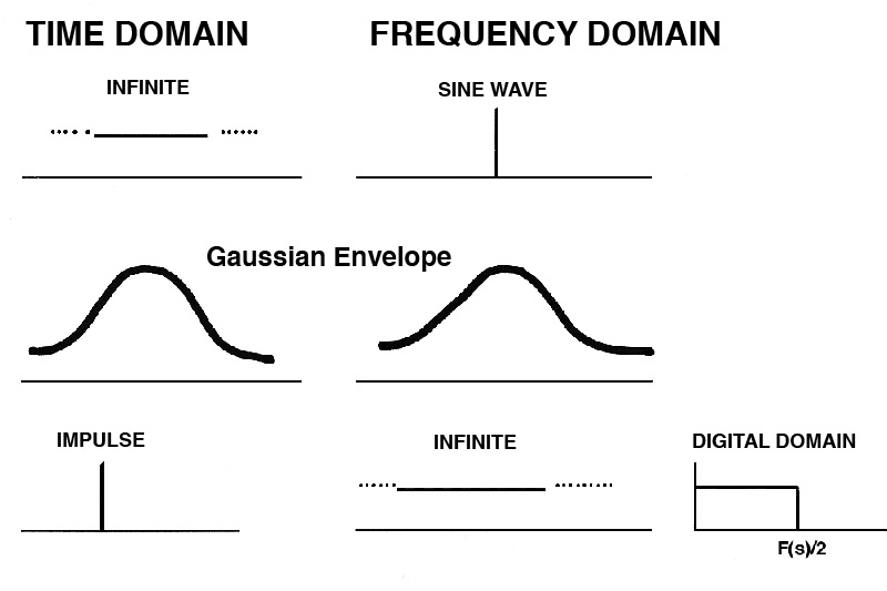
Speaking of sine waves, it is a useful mental exercise to consider the extremes of the frequency-time domain, as shown below, these extremes being a sine wave in the frequency domain (single frequency) and an impulse in the time domain (a pulse with theoretically no duration - try to imagine that!).
Theoretically, to get an absolutely pure sine wave, it has to have an infinite duration (another mind-bender). The “catch” is that when you start or end a sine wave there is a broadband click, and therefore it is no longer a “pure” frequency! Of course, if there were such a thing as an infinite sine wave, I suspect we wouldn’t hear it because it would always be there, and even the auditory system adapts to constant stimulation and the loudness response drops off.
Similarly, as the duration decreases to a pure impulse, the bandwidth increases to infinity – whatever that means! Fortunately perhaps, we don’t really have to contemplate what it means, because the digital domain is band limited to one-half the sampling rate, so it cannot represent extremely short impulses. As mind-bending as these extremes are, the point of the above diagram is that in the middle of this continuum, a Gaussian shaped envelope in the time domain has a Gaussian shaped spectrum.
Comparison of the time and frequency domains from the extremes to the middle
We encountered something similar in the Speech Acoustics module when we showed how the vocal tract departs from a perfect tube (which resonates at discrete odd harmonics) and its frequency response broadens into narrow resonance regions called formants.
In fact, there was enough psychoacoustic evidence in the 1930s and 40s that the Hungarian-British scientist Dennis Gabor in his 1946-47 publications was able to offer a critique that “Fourier analysis is a timeless description”. In fact, when we encountered the initial Fourier theorem its simplest form stated that a periodic waveform could be analyzed as the sum of a set of harmonically related sine waves, each with its own amplitude. But when such analysis was turned around to synthesis, the result was disappointing and static – precisely because it had ignored the time domain as Gabor predicted – and thus began a long and arduous task of incorporating time back into (re-)synthesis via complex temporal envelopes on each harmonic.
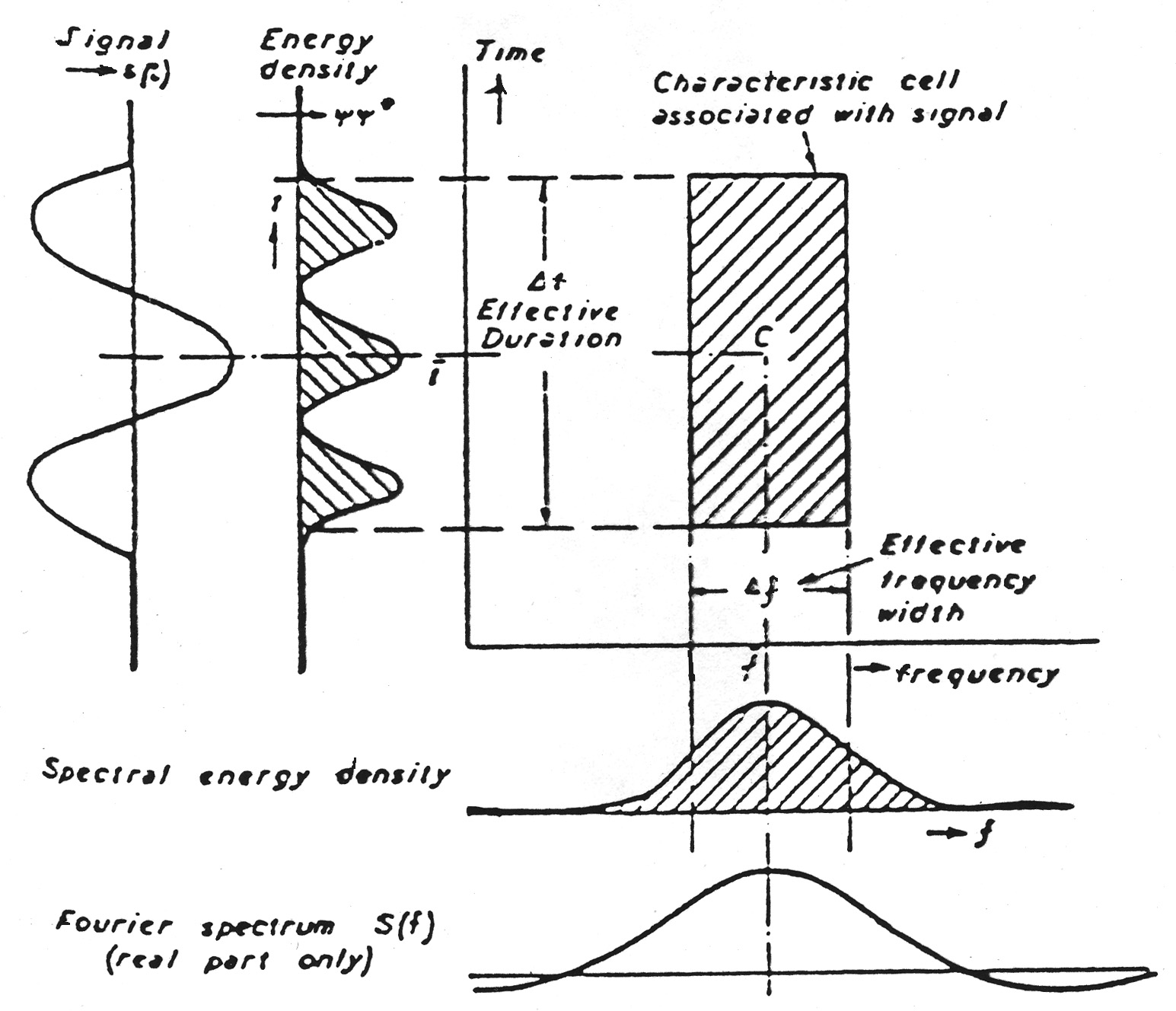
Original Gabor diagram of the frequency-time domain (click to enlarge)
Here above is the diagram that Gabor published in his 1947 paper in Nature (May 3, 1947, no. 4044) where he shows the time domain on the vertical y axis, and the frequency domain on the horizontal x axis. The shaded area is the quantum area or "cell" combining a short window of time Δt with its corresponding bandwidth Δf. That area cannot be subdivided (hence its quantum nature): if we decrease the time window (as in cutting a smaller portion of a sound) we increases its bandwidth and the sound gets noisier. Moreover, he shows that the time window Δt has a Gaussian shaped spectrum Δf. In this sound example, we hear a 20 ms enveloped sine wave become shorter until it is just 2 ms, with the corresponding increase in bandwidth.
A 20 ms sine wave is shortened to 2 ms and then back
(Click to enlarge)
This small windowed signal is sometimes called a “Gabor grain”, or simply a grain, which is a small particle of sound where, as an enveloped sine wave, it can be shown that it can theoretically be combined with other grains to re-constitute any time-varying signal.
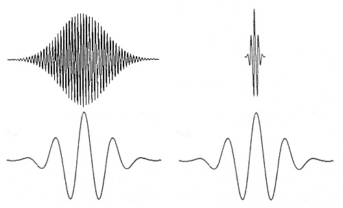
The following diagram shows at left a classic Gabor grain with a Gaussian envelope, a high frequency grain at the top and a low frequency grain at the bottom. On the right is a variant called a wavelet where the grain duration is inversely proportional to the frequency, so short in the highs, and long in the lows. In an actual analysis and re-synthesis of a signal, the use of wavelets is more appropriate.
Gabor grains (left), wavelets (right)
An analogy can be made to computer graphics where the grain is like a pixel, a small unit of colour out of which complex images can be created and which, most importantly, fuse together into a continuous image with sufficient density. Or one can recall the Impressionist painter, Georges Seurat, who experimented with a “pointillistic” approach in creating textured images composed of small daubs of paint.
So, why was this technique not immediately implemented in sound synthesis? After World War II, as electronic music synthesis began to be explored in depth, there were no grain generators available, just sine wave oscillators. Karlheinz Stockhausen famously began mixing them together in the Fourier manner (with harmonically related frequencies), despite his ear telling him they sounded like “little brutes” as he described them in a letter. His solution was to put these tone mixtures into a reverb chamber (which was available at the German radio) and used them in his Studie I and Studie II.
On the other hand, we now know that his teacher Dr. Werner Meyer-Eppler, from whom he had learned the Fourier theory, was aware of Gabor’s publication (he had a copy of it in his archive), but there was no method of implementing it at that time, the early 1950s. The closest would have the impulse generators that were also in the studio, and Stockhausen did use these at subaudio and audio rates to generate rhythm and spectra, respectively, which in fact illustrated the boundary between discrete and fused events which occurs around 50 ms (i.e. a frequency of 20 Hz).
As we known from pitch emerging gradually around the 20 Hz threshold, discrete (i.e. digital) impulses can fuse together to form a new, fused (analog) sensation called pitch, just as modulation at subaudio rates produces rhythmic effects until, around and above 20 Hz, pitched sidebands can be heard. A similar visual threshold for fusion also, remarkably enough, occurs around 20 Hz (50 ms), as evidenced in film frame rates. Below 20 per second, you can see a flickering image, as in very old films, whereas once there are the now standard 24 frames/sec, the image fuses smoothly.
Therefore, because of this perceptual threshold which is embedded in brain functions, the threshold for the microsound domain is described as 50 ms, below which audio events fuse, and above which they separate into separate rhythmic elements. And again, 50 ms is the periodicity of 20 Hz.
audio rate fusion <———> 50 ms / 20 Hz threshold <———> discrete events
Index
B. Granular synthesis. Synthesis involving the production of high densities of grains is called granular synthesis and traditionally refers to the use of synthetic grains, such as sine waves as building blocks, whereas we will use the term granulation in the next section when we want to refer to the granulation of sampled sound. Admittedly, the actual data may be stored identically in digital memory in both cases, but the control variables and the intent of the process are usually quite different.
Curtis Roads (inspired by Iannis Xenakis’ theoretical publications in the 1960s about the particle nature of sound and composing sound in "frames") was able to realize granular synthesis in non-real-time involving many hours of computing time in the 1970s. Real-time granular synthesis was first achieved by Barry Truax in 1985 using a microprogrammable DSP unit called the DMX-1000, controlled by a PDP mini-computer, which he used in his work Riverrun in 1986-87 (created with both sine-wave and frequency modulated grains). His real-time GSX software is demonstrated in this 2013 video from his studio.
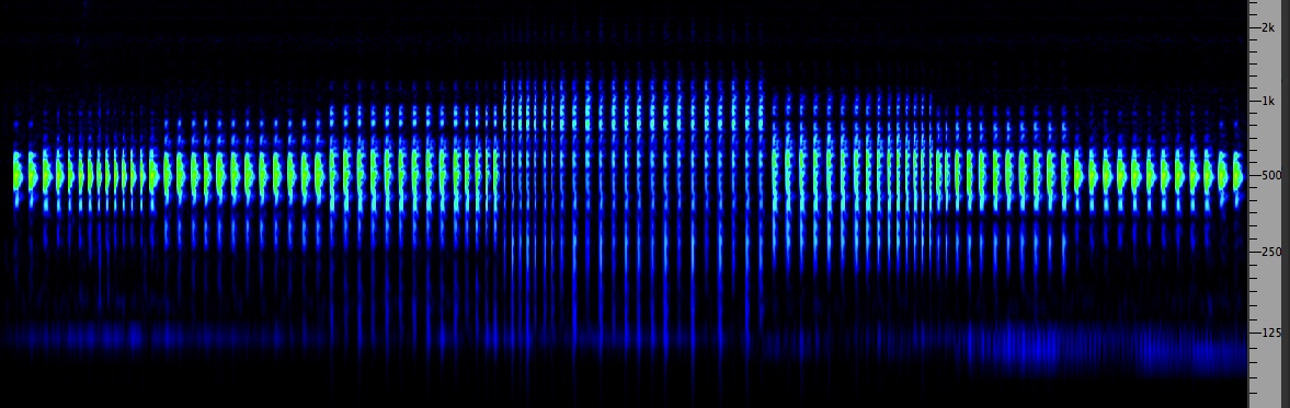
Here is an example of stereo granular synthesis from that period using sine wave grains, each with its own frequency, duration and waveform, where the choice of a particular frequency (and duration) is randomly made from a user specified range which in this case starts out as fixed, but then the average range ascends in frequency and broadens in bandwidth. What is remarkable – particularly given the static quality of sine waves – is the sheer power and volume of the resulting sound, in this case composed with about 1000 grains/sec, suggesting the analogy in Truax’s Riverrun of huge cataracts of water in a flowing river which develop from the insignificant individual droplets in the source.
Real-time stereo granular synthesis with increasing bandwidth of sine-wave grains
(Click to enlarge)
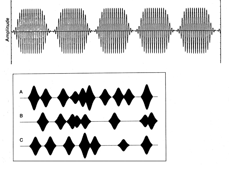
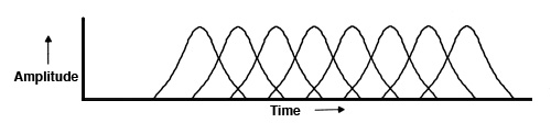
The required density of grains was achieved by programming 20 simultaneous grain streams that are sequences of grains separated by a specified delay time in milliseconds. This produces a type of granular synthesis known as quasi-synchronous because of the repetitions of grains. In the case of no delay (or a very short one), the result is an amplitude modulated grain stream, as shown below. However, in this implementation, the delay time could be randomized which simulated asynchronous granular synthesis where grains are scattered randomly, as shown below.
(top) Quasi-synchronous granular synthesis; (bottom) Asynchronous granular synthesis combining 3 streams
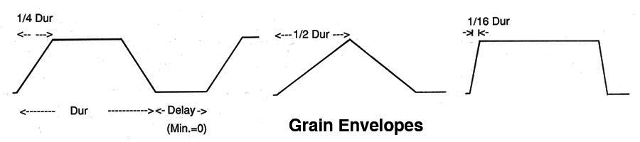
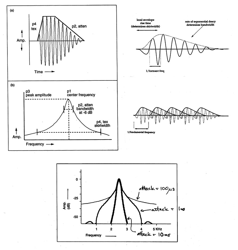
An additional feature of the GSX implementation is the control over the symmetrical linear grain envelope shape, with the attack and decay identified as a fraction of the total duration. Again, as is typical in the time-frequency domain, a sharper attack produces a broader bandwidth, and a soft attack (e.g. 1/2 or 1/4 of the total grain duration) results in a narrower bandwidth in the resulting spectrum. Note that linear amplitude envelopes are used, rather than trying to replicate a Gaussian curve, as they require less calculation and produce a very similar effect.
Take home message: with microsound, a change in the time domain results in a change in the frequency domain
The granular concept of a basic enveloped building block of sound, the grain, has been elaborated in a variety of synthesis approaches. Curtis Roads, in his book Microsound, documents the pulsar, glisson, wavelet, trainlet and other varieties of micro-level synthesis based on grains.
Also, grains can be organized other than stochastically, one alternative being a mapping to a non-linear dynamic system, popularly called a chaotic function or "chaos", as shown here.
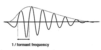
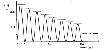
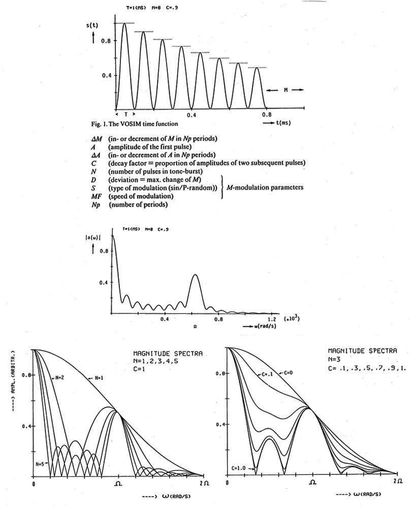
Given the formant-like nature of the grain spectrum, it is not coincidental that at least two vocal synthesis methods are based on a similar concept: the FOF method (referring to the French forme d’onde formantique, that is, formant waveform), based on an asymmetrical damped sinusoid, and the VOSIM vocal simulation model, based on a sine squared pulse, as shown here.
FOF basic unit and spectrum
VOSIM basic unit and spectrum
Index
C. Granulation of Sampled Sound. As mentioned above, we will refer to the processing of sampled sound by separating it into grains as granulation, as distinct from granular synthesis itself which uses synthetic grains and because of their simplicity, requires a lot of control information in order to give them a dynamic shape. With granulation, the richness of the sampled material provides most of the interest in the processing.
All methods of stretching (or compressing) a sound in the time domain without changing its pitch use a windowing technique to achieve the desired result. In a waveform editor, it is assumed that you want such an adjustment to the duration of a sound to be transparent (i.e. with minimum artifacts). This is quite difficult to do, but given the demand for it, sophisticated algorithms are used to overlap windows of the signal keeping the phase information intact and the stretch barely noticeable.
However, this approach has a major limitation for the length of the stretch that is possible to achieve without generating artifacts. To lengthen a sound by, say, a factor of two, you are going to have to repeat samples twice, and more times than that for even larger stretches. This produces the characteristic amplitude modulated effect in the audible range, as shown in the above diagram for quasi-synchronous granular synthesis. In this sound example we use a phrase, heard first at the original speed, then stretched by 1.5, 2, 4, and 8 times the normal length. The 1.5 extension is still acceptable, but after that, the modulation becomes noticeable and increasingly objectionable.
Spoken phrase at original speed, then stretched by 1.5, 2, 4 and 8 in an editor
Source: Thecla Schiphorst
One technique that works well for periodic sounds, is pitch-synchronous granulation, as shown here, where the grain envelopes line up with the periodicity of the signal.
As mentioned (and shown) in an earlier module, the Springer Tempophone (Tempophon in German, also Zeitdehner, time stretcher, or Zeitregler) was an early analog form of time stretching with a rotating set of heads that essentially picked up “windows” of sound on tape from each playback head and overlapped them. It was mainly used to change pitch without modifying the duration, but in a separate mode of operation where the tape speed changed, it could also stretch the sound while maintaining the same pitch. The theory for this analog version of granulation was also established by Gabor, who built an optical soundtrack version of it with a film projector in 1946.
Pitch-synchronous granulation
A more creative and flexible approach to digital sound processing is what we are referring to here as granulation, which deliberately adds a texture to the sound through the overlapping (or detached) grains taken from neighbouring or even distant parts of the signal. Multiple streams of grains combine to provide such a texture, each with its controllable grain envelope, duration and shape. With this technique, there is no theoretical limit to the stretch, but keep in mind that stretching a second of sound by a factor of 1000, is going to last over 15 minutes!
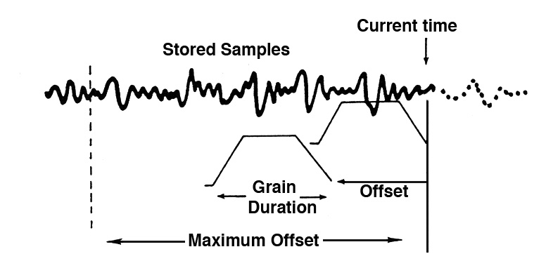
But how does granulation work to avoid changing the pitch of the material? In this diagram, we see a general solution involving making the “current time” position within the signal move forward independent of the overlapping grains which always take their samples in the same order as they were recorded, hence no pitch change. But the current time can move forward (or backwards) at any desired rate.
Time-stretching model with no pitch change implemented with windowed grains
The diagram also shows that the grains can be taken from anywhere in the recent past (since all of the samples are in memory). There is no standard term for this distance, but in this diagram it is called an “offset” which can be different for each sample. The smaller the offset, the closer all samples will be to the current time, but if the maximum offset range gets larger, then the samples could be taken from the next syllable, creating a stuttering effect, or even from a more distant part of the sample, making the output sound quite jumbled.
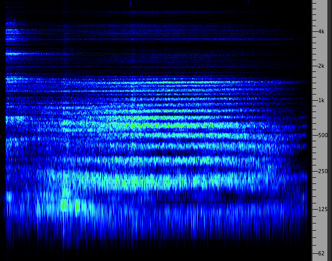
Using a short sample. In certain kinds of sampled sound, and the voice in particular, there can be a lot of variation within a very short sample. In this case, moving the grains slowly through the sample acts as a kind of aural “microscope”. In The Wings of Nike (1987), there are only two short phonemes used as source material, a male phonemic sequence from the word “touch”, and a female phoneme on the vowel “aah”. Each lasts about 170 ms. In the first example, the grains move through the male phoneme sequence very slowly, coming out of the consonant “t”, through the vowel (the short “o”), and heading towards the final sibilant consonant “ch”.
Male phoneme from the word "touch"
Source: Norbert Ruebsaat
Granulated male phoneme, moving slowly through the sample
Female phoneme "aah"
Click to enlarge
In the first movement of the work, these two stretched phonemes, plus octave transpositions up and down, are the main sound material. But even in this highly stretched state, the vocal phonemes can still be identified as male and female, but they appear larger than life and create a sonic environment of their own.
Opening of The Wings of Nike using stretched male and female phonemes
(stereo reduction from 8 channels)
from CSR-CD 9101 Pacific Rim
Click to enlarge
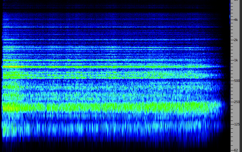
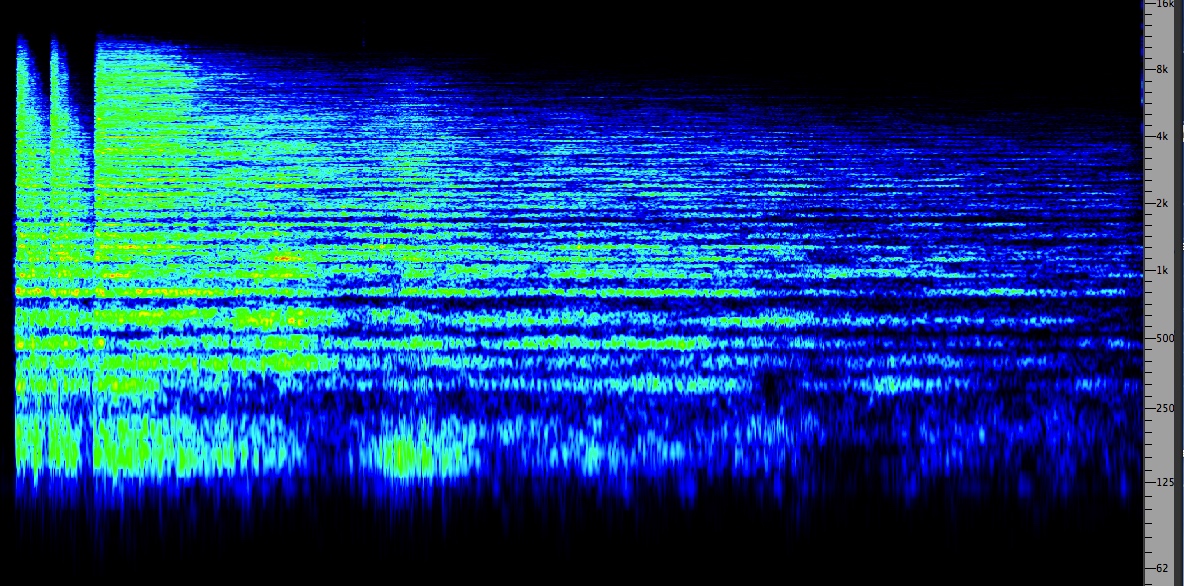
The source material in the next example is a bit longer, and consist of three blasts of a British Columbia ferry at Horseshoe Bay in Vancouver. This ferry terminal is below the rock face of a high mountain, so there is a great deal of reverberation. We first hear the original blasts, then the next recording is the granulated version, with the first two blasts not stretched, and then the final one and its long decay highly stretched (20 times).
Notice how you can hear the details of the spectrum of the horn on the third sound, whereas it is the sharp attack of the first two that is clearest. Prolonging the final decay also gives you time to savour the intricacies of the reverberation. You are essentially switching from focussing on the temporal envelope (and identity) of the sound at the start to a mode where you seem to be listening “inside” the sound and its spectrum during the remainder.
The paradox here is that by linking frequency and time at the micro level of the grain, you can separate them at the macro level!
Three ferry horn blasts (original)
Source: WSP Van 39 take 4
Granulation of the three horn blasts, stretched 20:1 on the third blast
Click to enlarge
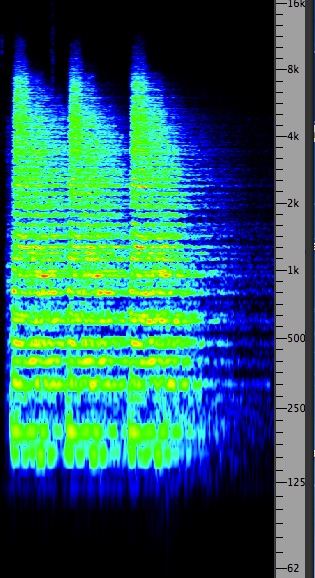
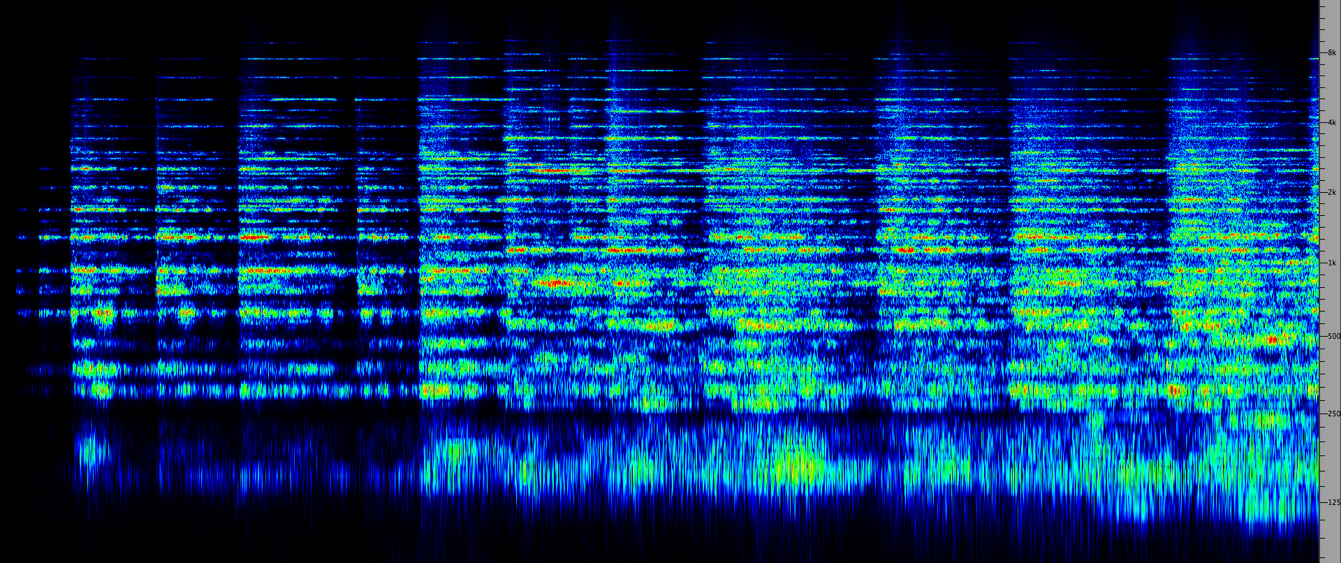
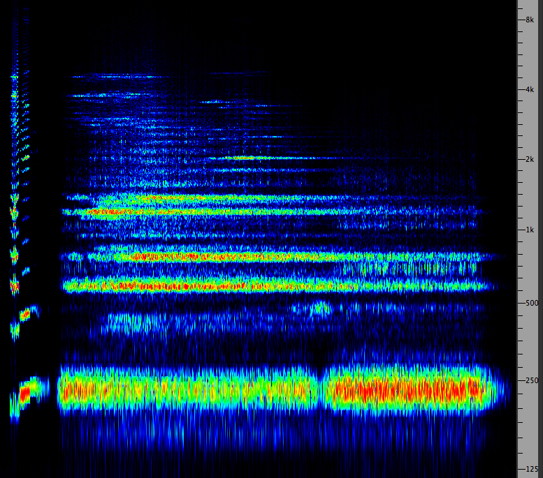
Composing with a longer sequence. Sometimes a recording such as the next one seems to provide enough material for most of an entire work. This is the case with a recording of the bells of the Basilica of Notre Dame de Québec from 1973. The sequence is of just three bells, being sounded in the European style that starts with the highest bell, then adds in the lower ones in turn. An interesting counterpoint always ensues where the bells ring at their own pace, so the overall pattern, even with just three bells, is constantly changing.
In stretching the sound of the bells, often 20 times or more, their volume is greatly enlarged, such that their resonances start sounding more like reverberation inside the church itself. In fact, the actual church is relatively small, but once the bell sound is stretched, it begins resembling the acoustics of a much larger edifice. The traditional form of a basilica is that of a cross within a rectangle, and so the opening of the piece, with the lengthy stretching of the bells, represents the long nave that one encounters on entering the church.
Although the bells have a rich spectrum on their own, they still occupy a limited range of the frequency spectrum. Therefore, to augment their spectral volume further, two transpositions were added, one octave down and the interval of the 12th up (an octave plus a fifth). Particularly in the 8-channel version, the high frequency portion of the spectrum seems to come from harmonics swirling above one’s head high up in the ceiling area.
Three bells from the Basilica of Notre Dame de Québec (original)
Source: WSP Can 60 take 2
Opening of Basilica (1992)
from CSR-CD 9401 Song of Songs
Click to enlarge
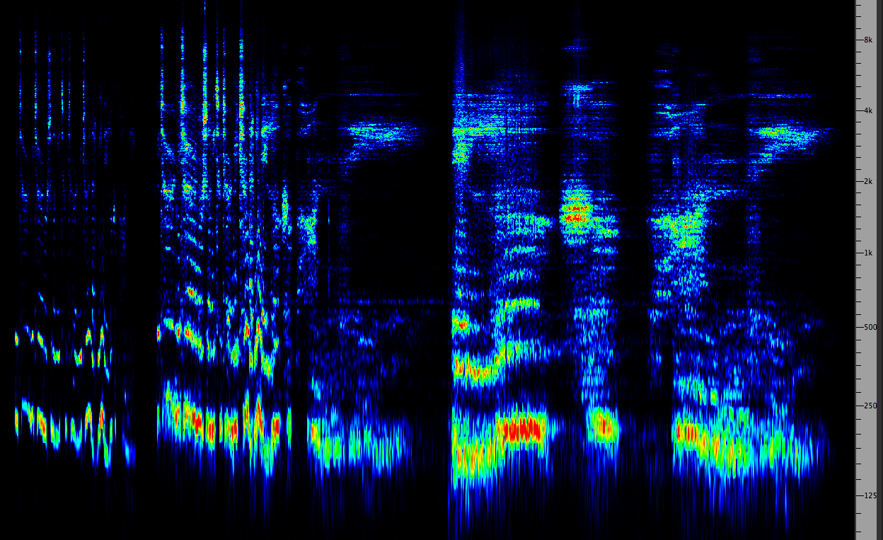
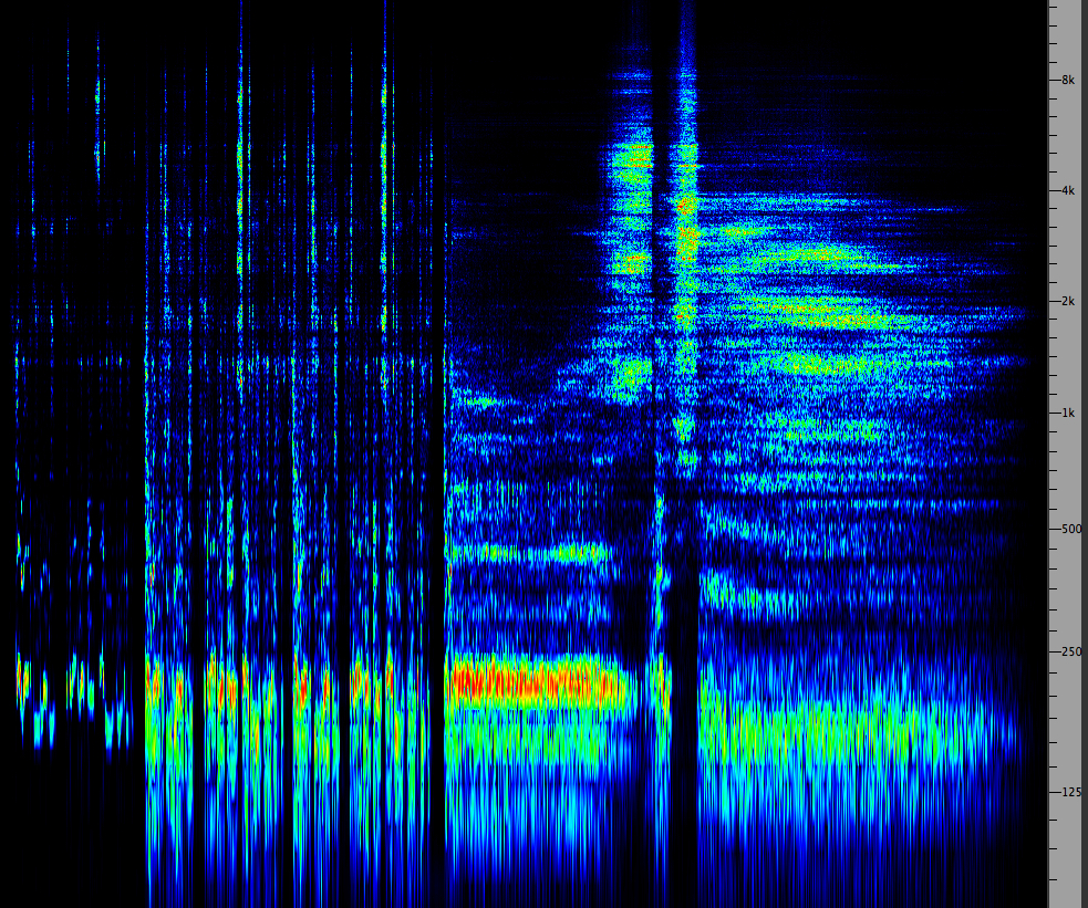
Text-based work. Because of the density of phonemic information, as can be seen in a sonogram, and our sensitivity to spoken language in general, it is often interesting to use granular time-stretching with speech material. Here are some examples from Song of Songs (1992), based on the famous Song of Solomon text from the Old Testament.
In the first example, the musical pitch inflections found in the original reading become even clearer when stretched and more song-like. Small stretches (2:1) on key words such as “return” and “look” gave them more emphasis in the rhythmic flow, with the end of the phrase stretched by 10:1. The vowels provide the main pitch interest, but the noisy bands of the consonants (many of which can’t be stretched in normal speech, except for the sibilants) sound much noisier and possibly too harsh.
Song of Songs text (original, then granulated with small stretches and finally, stretched 10:1)
Source: Thecla Schiphorst
Click to enlarge
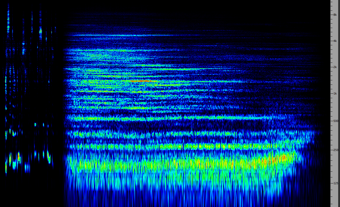
In the second example, the particularly musical reading of the “Rose of Sharon" text is enhanced, not only by an initial 33% stretch, but by harmonizing it with lower pitches at intervals of 4:3, 4:2 and 4:1 below the normal pitch (the fifth, octave and double octave below), placing it in the male vocal range and blurring the apparent gender of the speaker. Also note that "harmonizing" the consonants produces some strange effects.
After the second repetition of the text, the word “Rose” is stretched by 50:1 with the same harmonization, and the final word “Sharon” by 100:1, essentially turning it into an ambient or environmental sound. This blurs the distinction between the human voice and the natural sounds that accompany each of the movements of the work, and reflects the original text that compares the beauties of the beloved to those of nature, and vice vera.
Song of Songs text "I am the Rose of Sharon"
(original, then harmonized and granulated with small stretches and finally, stretched 50:1 and 100:1)
Source: Thecla Schiphorst
Click to enlarge
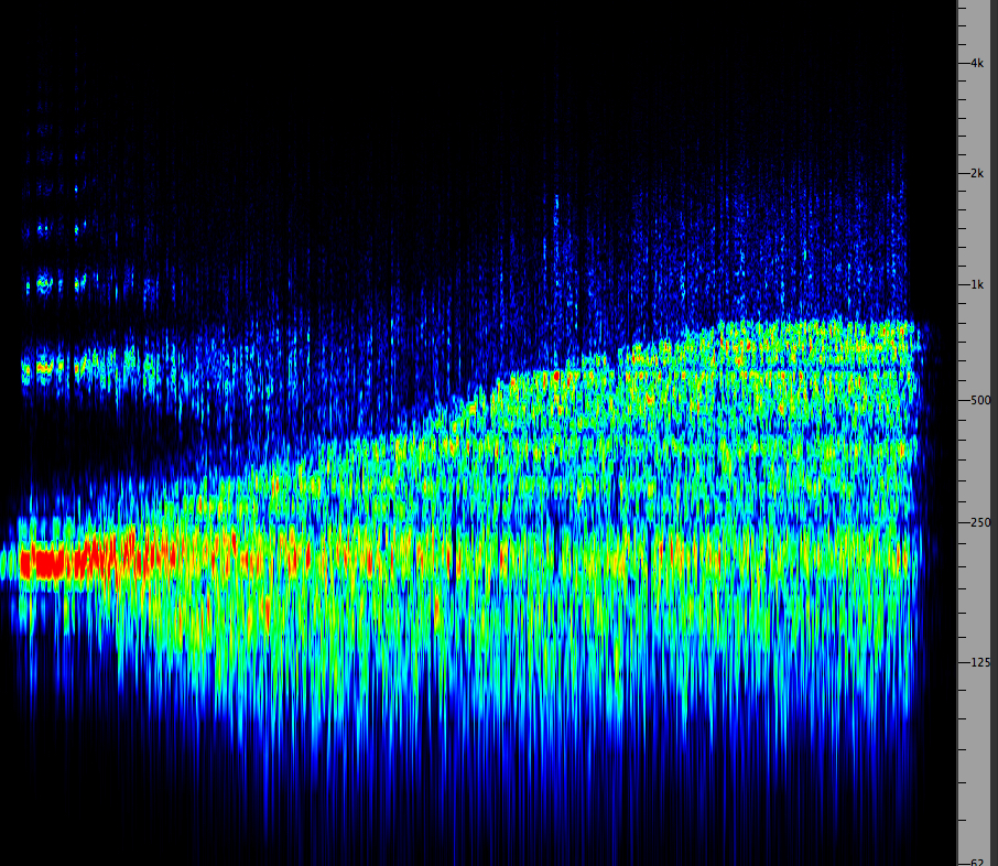
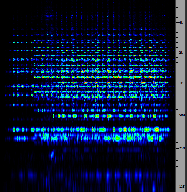
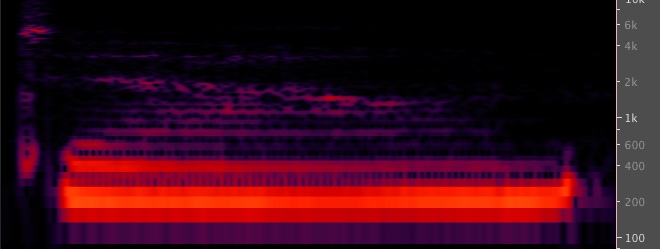
In the final example, a single word “down” with its characteristic downward sliding diphthong “ow”, is given a mega-stretch of 60:1 and 100:1, along with the same harmonization as in the previous example, plus an upward 3:2 (fifth) harmonic, thereby producing a huge chord. The spectrum of the brief phoneme is also included in the left diagram below. The original text is given first just to show how brief the word “down” is.
The word "down" stretched and harmonized (original text, then granulated with 60:1 and 100:1)
Source: Thecla Schiphorst
Spectrum of "down"
(Click to enlarge)
Click to enlarge
Stretching Processed Sound. When processing brings out the inner richness of a sound or sound mix, stretching the sound afterwards allows that richness to be heard more clearly in a reflective manner. The three examples here begin with sound that has been first resonated, or auto-convolved and resonated, and in the last example, auto-convolved and mixed in 4 different pitch ranges. In each case, the inner complexity of the processed sound is made more evident through the stretching.
In the first example, the mezzo-soprano singing voice has been strongly resonated prior to stretching, moreso than one might normally do, but once stretched, the resonance is smoothed out and becomes closer to reverberation.
Mezzo soprano voice in Temple (2002),
original, then resonated and stretched
Source: Sue McGowan
Click to enlarge
In the next example, three piano arpeggios are heard in their auto-convolved state, which already doubles the length and smooths out the attacks, prior to being stretched further.
Three piano arpeggios in From the Unseen World (2012),
auto-convolved, then stretched
Click to enlarge
Finally, an eagle cry has already been auto-convolved and mixed in four different pitch ranges (the original, and each of three octaves below) such that each downward octave doubles the duration, and then is stretched again.
Eagle cry mix in The Garden of Sonic Delights (2016),
auto-convolved, then stretched
Click to enlarge
Index
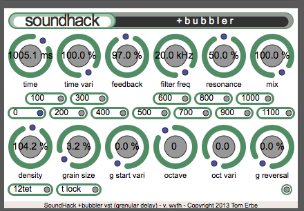
D. Studio demo’s. There are a variety of programs that use a granular approach to processing without time-stretching, and these are useful for allowing the user to add texture and density effects to a sound. These programs include SoundHack’s Bubbler plug-in (part of the free Delay Trio download) and GRM Tools Shuffle module. They basically extend the delay line approach as covered in this module by allowing grain envelopes to be added to the sample.
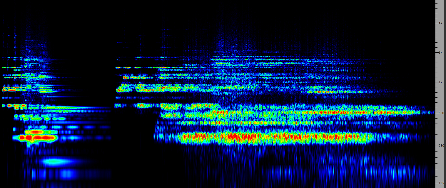
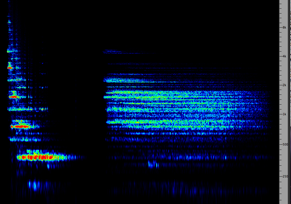
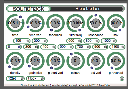
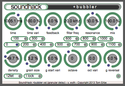
The SoundHack Bubbler adds a “time variable %” to the delay time that functions similarly to the “offset range” introduced above. That is, the delay range can be used to specify where in the overall sample the grains will be taken. The first example shows a small 10% range, resulting in a kind of stuttering effect with the text still recognizable, and in the second example, a full 100% range is used which jumbles the entire signal.
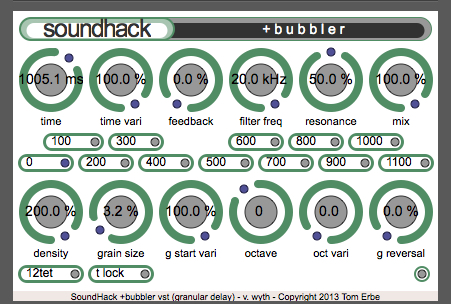
The density parameter adjusts the amount of overlap between the grains, where 100% indicates that an average of two grains will be present at any time, with more detached grains nearer 0% and a higher density at 200%. The all important “grain size” is a percentage of the overall delay time, in this case kept at 3.2% of the current delay time. In these examples we have used a short text, since the effects are much more noticeable that way when you are first learning how to use the software.
The density parameter adjusts the amount of overlap between the grains, where 100% indicates that an average of two grains will be present at any time, with more detached grains nearer 0% and a higher density at 200%. The all important “grain size” is a percentage of the overall delay time, in this case kept at 3.2% of the current delay time to produce short grains. In these examples we have used a short text, since the effects are much more noticeable that way when you are first learning how to use the software.
Text granulated with short offset range
Text granulated with large offset range
Text granulated with large offset range and feedback
Text granulated with large offset range and higher density
In the third example, there are similar settings but with a large feedback component. As in other contexts we’ve looked at, the feedback gets cut off at the end of the sample when the processing is applied, and therefore silence should have been added to the original sample. The other variables function similarly to the delay line app, except for the “grain start variation” which represents departures from periodic or quasi-synchronous repetition.
In the last example, the grain start variation and the density are maximized to produce a very stochastic effect, which with the large offset range turns the text into a smooth phonemic texture.
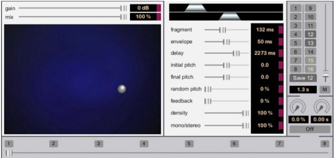
The GRM Tools Shuffle module performs a similar type of granulation without time-stretching, but with a very different graphic interface. The grain size is on the vertical axis, with short grains at the bottom, and the horizontal axis controls the delay time, with short delays at the left, and up to three seconds on the right. The visual display of the envelope at the top right is very effective in showing what is happening. When combined with the density parameter, both granular and macro-level effects can be generated, along with the other parameters listed.
GRM Tools Shuffle
Granular Time-stretching with MacPod. One of the most flexible and user-friendly granular time-stretching apps is MacPod, created by SFU alumnus Chris Rolfe. It was designed for the Mac back in the 1990s (and won a software award from the Bourges Competition in France) at a time when performing sample-based DSP processing was very difficult. Today it is available as a free download for Mac or PC from thirdmonk.com (contact the author for current availability).
Note that it has a “record to disk” option so it can operate stand-alone, independent of an editor or DAW. The recording only starts once the “play” button is pressed, and ends with the “stop” playback button. This means you can improvise as long as you like, and then edit the best parts of the file in an editor later.
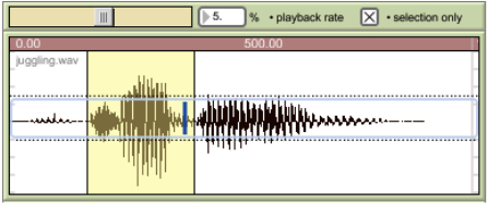
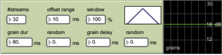
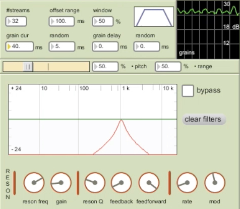
In this first video demo, we will load the same vocal text file we used in Bubbler, and perform a simple manually controlled stretch operation. The entire sample will be used (unlike the “selection only” version shown at the left). For the granular parameters, shown at the right, we will choose some fairly “neutral” values (not those shown here), such as a grain duration of 40 ms (just below the fusion threshold of 50 ms to avoid any pulsation of the grains), a small random duration range (5 ms) to avoid any modulation effects, the smoothest window (100%) conveniently shown in a small window, no grain delays or equalization. These grain parameters might be saved as the first preset for later use. Also note the real-time sonogram similar to what we have been showing here.
Sample window
grain parameters
Video demo
In the bar above the sample window, once we start the playback, we will hear the stretching occur as soon as we move the cursor away from 100%, small stretches at first, then to the maximum stretch of 1%, or “frozen” at 0%, or with a backwards movement through the sample at negative values. The manual control is very responsive to your mouse movement and it is relatively easy to impose longer durations on significant words, such as “rose, lily, valley” in this example, then end with a very long stretch on the final sibilant.
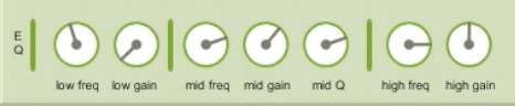
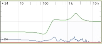
In the second video demo, we add some different parameters and options. First of all, we have added a simple EQ to the sample, mainly to remove low frequencies, by lowering the low frequency gain and adjusting the cut-off frequency. These are the green knobs and green line in the spectrogram window which makes it easy to co-ordinate the EQ with the actual spectrum (in blue). This high-pass effect is useful because when you window low frequencies with grains, their bandwidth is also broadened, as predicted by the time-frequency domain theory as above. We also added a small EQ boost around 3 kHz with a medium narrow Q value.
EQ parameters
Spectrogram (with green EQ setting)
We have also changed the grain parameters in this demo to a grain duration of 25 ms (to add some spectral broadening to the voice), and some random delays from a 50 ms range (to add some texture), and a modest 100 ms offset range for the same purpose, with grains sometimes being taken from neighbouring phonemes.
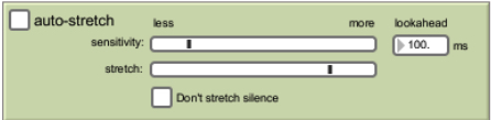
However, the main point of the demo is to illustrate what is arguably the most unique and useful option in the program, the “auto-stretch” function as shown at right. It correlates the stretch function with the sample amplitude, something that we could only do quite generally with the manual control. This function can “catch” momentary peaks and slide over the quieter parts, including the check box for not stretching silences (you don’t think you’d need that until you hear what happens without it).
Video demo
Auto-stretch controls
The main controls for the auto-stretch are the two bars for degree of sensitivity to the correlation, and the overall amount of the stretch. Careful adjustment of both of the these is needed to get the right effect, particularly with speech where the signal level is changing all the time. In this case, we tried to adjust it so the consonants wouldn’t be stretched as much (luckily they weren’t that strong in amplitude) and the stressed vowels would be given a greater stretch. Watching the stretch bar’s behaviour is very useful for seeing what is happening, as well as hearing it.
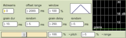
In this third video demo, we treat the voice more abstractly and create very small grains (10 ms with a 5 ms range), starting with a fixed delay (250 ms) to provide a regular rhythm, expanded later to a random range of 100 ms. The offset range is 2000 ms (2 sec.) which allows grains to be taken from a wide range of the sample. However, we start with 0 voices, and slowly bring them in manually. This is an attractive alternative than an amplitude fade, or a linear density control. The new grain streams will likely be out of synch as they begin, however note that they come in evenly on either the left or right channels to provide a good stereo image.
To make the transition more efficient, the initial set of grain parameters has been stored as preset 2 (with 0 ms delay range), and as preset 3 (with 100 ms delay range) which is triggered part way through. Note that the transition from preset 2 to 3 is 1000 ms (1 sec) which can be seen as a ramp. These presets can be stored in a file with the “write” button and retrieved with the “read”. Note that the preset also includes the fade time and auto-stretch settings, so very complex transitions can be performed.
Video demo with short grains;
initial parameters at right
Once the full texture is achieved in this demo, the attack of the grain envelope is manually changed from its initial “soft” value of 100% to a final value of 16% which broadens the bandwidth considerably. The sequence ends with the grain streams dropping out again one by one. The sound file itself is stretched at a constant 40% rate, just enough to bring in new phonemes. However, the offset range is set very high (2 seconds) so there is no continuity to the text at any point.
As an alternative, you could try this with a decreasing offset range, such that the text might start appearing again before it “evaporates”. However, I expect a much longer delay time (e.g. 1000 ms) should be used, and as streams are brought in, the offset range needs to be reduced.
When you want to change grain parameters, you can drag their value up or down, or you can click on the box and simply type in the desired value for a sudden change. Given the micro time nature of granulation, there are cases where you may need a decimal place, so if you position the cursor to the right of the period, you can get up to 3 decimal places. For instance, in a more static amplitude modulation situation, this can change the modulation frequency more smoothly.
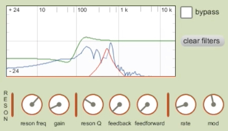
The fourth video demo takes a very rich sound as its source, the large Salvator Mundi bell from the Salzburg cathedral in a short solo ring. We will use this opportunity to show how to add a resonance filter to the output stream. The controls are colour-coded in a reddish orange, and the diagram below shows the one we settled on for the bell (in addition to the high pass EQ). The resonant frequency was set in the range above 800 Hz (and displayed in red) where numerous upper partials occur in the bell.
A fairly low gain was applied as it doesn’t take a lot of boost to bring these forward, and at the right we added a very slow modulation of the resonant frequency so that it spanned about an octave. This slow modulation rate was set to approximately match the tempo of the ringing. The auto-stretch function was also used and adjusted as you can see in the video. An offset range of 200 ms gives a slight stutter to the attack.
Video demo stretching a large bell;
resonator parameters shown at right
In our final MacPod demo video, we show some additional parameters provided by the program, along with more live interaction during the playback. We start with the configuration of the resonator as suggested in the MacPod manual (pp. 8-9) for a “flanger” effect. This involves two parameters called “feedforward” and “feedback”. These refer to circuits that we encountered in phasing where the feed forward version combined the input signal with a time delayed version of itself, and the feedback version added a resonant pitch. We will set the values as suggested in the manual, but reserve the more powerful feedback one for real-time variation during the sound.
The sound chosen is the high-pass scything sound introduced in the filter module, except that we will transpose it down by 50% in the bar above MacPod’s Spectrogram, and add a 50% pitch variation as well to thicken the bandwidth of the sound. The offset range of 100 ms enhances the stereo effect. The stretch factor will be left at 10% to make it very slow, and allow it to combine well with the resonance modulation suggested in the manual (a .24% rate and 20.5% modulation amplitude).
Video demo stretching scything sound with interaction;
grain and resonator parameters shown at right
During the playback, we will alter three parameters in order to add a variation to the otherwise repetitive nature of the sound: (1) feedback percentage, that adds a spectral pitch; (2) grain duration, going from 40 ms to much shorter values, to add bandwidth; (3) grain delay range, going from 0 (thickest texture) to higher values to loosen the texture. The direct-to-disk function will record everything we do. The resulting image should be that of gusts of wind, perhaps whistling through a shed.
Index
Q. Try this review quiz to test your comprehension of the above material, and perhaps to clarify some distinctions you may have missed.
home