|
DYNAMICS |
Dynamic Range and Compression
|
DYNAMICS |
The term "dynamics" in the electroacoustic context always refers to patterns of amplitude and intensity, and therefore is related to loudness. However, it is not identical to loudness as the psychoacoustic response to intensity, as discussed in the Magnitude module. Nor is it necessarily the largest component in perceived volume which has a strong spectral and spatial component.
Yet, the control over dynamics and dynamic range is one of the most important variables in an effective mix, and not just in the commercial world where there are more or less standardized techniques for using compression and expansion techniques in mastering.
We will discuss the topic in the following sections.
A) Dynamic range
B) Compression and expansion
C) The historical uses of compression in broadcast and recording media
D) Examples of bad compression
E) Studio demo's of dynamic range control
P) Downloadable pdf summary of Dynamic Range and Compression (control click or right click to download)
Q) Review Quiz
home
A. Dynamic Range. We can speak of the dynamic range of a sound or sequence of sounds, and we can also refer to the dynamic range of a storage or reproduction medium. In each case we are referring to the range of amplitudes or intensity from the lowest to the highest. These ranges can be compared with the dynamic range of hearing itself, which is usually described as 120 dB, going from the threshold of hearing to the threshold of pain or discomfort.
However, as discussed in the Magnitude module, this large theoretical range of dynamics in hearing is not always available to us, as the auditory system is constantly adapting to ambient conditions which create a threshold shift. We can make a simple comparison to different levels of light to which the iris in the eye reacts by getting smaller in bright light, and larger in low light conditions. And we are familiar with the time it takes to make transitions between those conditions. Normal eyesight can adapt over time to large changes in illumination – unlike most optical systems used in photography and video which do not normally reproduce the large range of light energy we are capable of seeing.
Similarly, we adapt our hearing to a given range of sound intensities that we are currently hearing, probably with a maximum range of about 60 dB or less at any given time. And it takes about the same time to adapt to low level sound environments as it does to those with low illumination. There is also a corresponding relativity in our loudness response. Quiet sounds at night may suddenly seem very prominent, and even loud, whereas they would barely be noticed in more typical ambient situations.
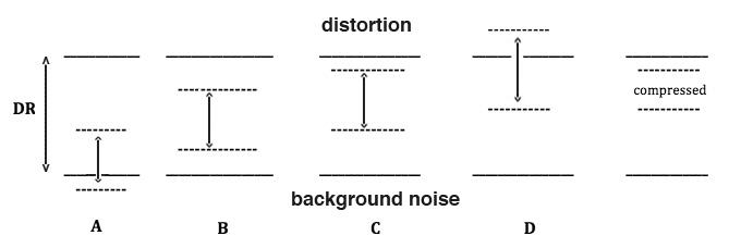
So, when we record a sound sequence, we have to choose the appropriate recording level, as discussed in the Field Recording module. We want the sound to be clearly distinguishable above any noise in the recording system, but not so strong as to become distorted. In other words, we have to fit the dynamic range (DR) of the sound within the DR of the recording medium. Consider the following 4 cases, A through D. The solid lines give the DR of the medium, and the dotted lines give the DR of the sound signal, boosted from a low recording level to a high level. Which is the best choice?
Comparison of recording levels within the available dynamic range (DR)
Clearly in case A, the recording level is too low, and the quiet parts of the sound get lost in the background noise. And in case D, the peaks of the sound go above the distortion level. But which of the remaining cases, B or C is best? Both avoid distortion and keep the quiet parts above the background noise, but case C is better because it gives the entire signal the best signal-to-noise ratio.
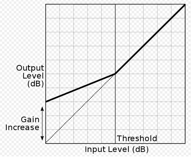
However, we can still rescue case D, by reducing the dynamic range of the signal through the process of compression. Notice that the peak levels have been reduced such that they “fit” within the DR of the medium. The overall loudness of the compressed signal will also be greater because it “rides high” in the DR of the medium, as it is usually expressed. We will describe the process in detail below, but here is the general idea of how gain reduction in the peaks can be achieved. Higher input levels past a certain point (the threshold) are reduced by a certain ratio.
Compression in dynamic range
There are also cases where the DR of the medium is simply too small. It is estimated that the first electrical recordings in the 1920s, the 78 rpm shellac discs, had a DR of only 30 dB (and a maximum duration of about 4 minutes, a duration that influenced the songs that were recorded on it). The long-play vinyl record introduced in the late 1940s, enlarged the DR to about 57 dB, and the duration to about 30 minutes.
Optical sound tracks on film, and early video formats had a very low DR, perhaps about 40 dB, whereas the best tape recording formats could exceed 60 dB, even without noise reduction. So, compression was necessary to fit a sound mix that was mastered on tape onto these audio-visual formats.
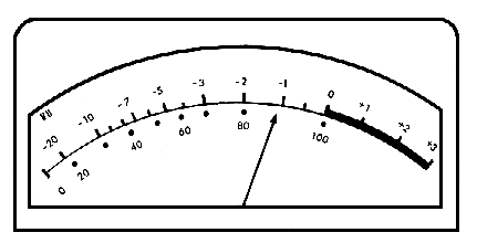
The levels of analog signals were monitored on a VU meter, as shown below (where VU stands for Volume Unit). Note that the highest distortion-free level was labelled 0 VU, with other signal levels measured in negative dB below it. However, analog tape did allow some headroom, that is, it could accurately record momentary peak levels above 0 VU with no audible distortion. Still, it was not wise to overly rely on that option, and the ballistics of the VU needle usually meant that these peak levels could be seen to be brief.
Analog VU meter
However, digital audio representation, as discussed next, has no theoretical headroom because it lacks the number of bits required to portray numbers larger than the maximum. In practice, most applications show a red warning signal when an overflow is imminent or has actually occurred since the “ceiling” is fixed.
As documented in the Sound-Medium Interface module for the digital representation of sounds, the DR of digital audio was greatly increased in the late 1970s and 80s based on the number of bits used. The rule is that each bit (which doubles the size of numbers that can be represented) increases the DR by 6 dB. Therefore 16 bits should theoretically provide a DR of 96 dB. This figure is theoretical because, as also shown in that module, the least significant bit is basically quantizing noise, so 90 dB is a more likely figure.
The part of the digital sound that is most sensitive to DR is the end of its decay, or a very quiet sound passage. With environmental recordings, there is always an ambient component at the low end of the DR, so the end of a decay or reverberation is not as noticeable. But in a studio recording, one can argue that a 24 bit format is preferable. We also encountered the special case of convolution, and auto-convolution in particular, where a large dynamic range is involved with its multiplication of spectral energies, and 24 bits is absolutely necessary.
So, here is a paradox. Given the enhanced dynamic range of digital audio, why is it seldom fully used? That is, why are commercial recordings, particularly of popular music, always consistently loud because of high levels of compression? In fact, in the last decade, critics have referred to “loudness wars” in describing extreme uses of compression. This is a large and controversial topic, and we will return to it in section C to provide some historical context. But first, in the next section we will present the theory of dynamic range control via compression, expansion, limiting and gating with sound examples of their use.
Index
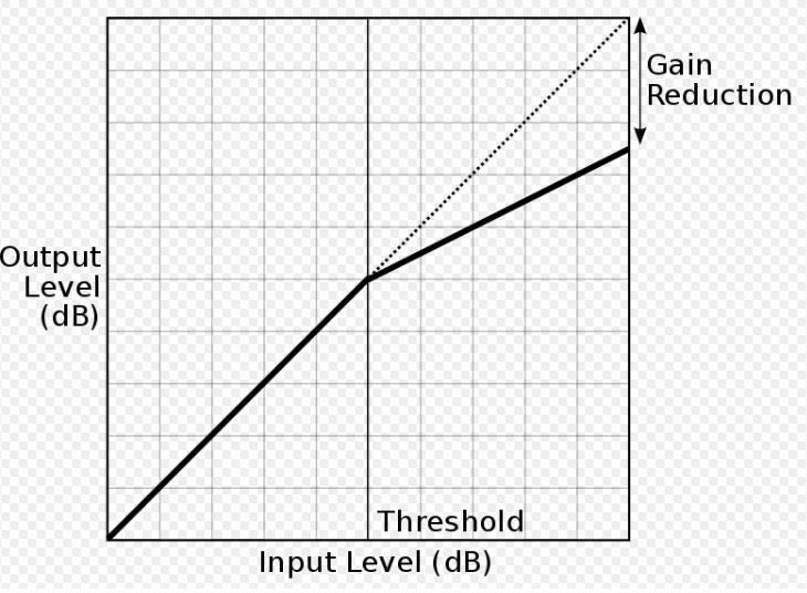
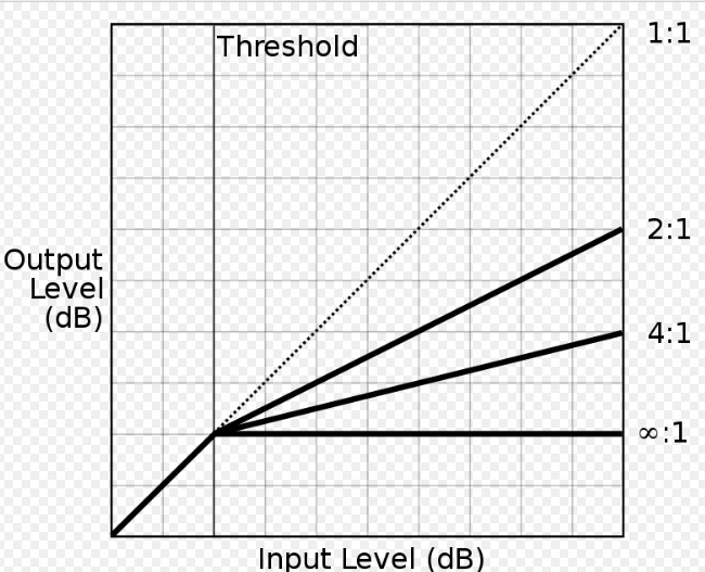
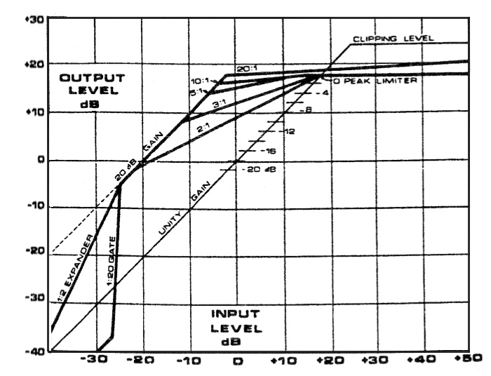
B. Compression and Expansion. The traditional methods of controlling dynamics in a signal are usually explained with reference to a graph such as the one below. This is a classic response diagram where the output (y-axis) is mapped against the input (x-axis). The reference point is the diagonal line called unity gain, which means there is a one-to-one (1:1) relationship between input and output, that is, a linear relationship where the ratio of low to high levels in the input are mapped onto the same range of levels in the output. Non-linear amplification, expressed as a ratio, such as 2:1, 3:1 or 4:1, above a threshold point, is shown as increasingly flattened lines.
Compression with different compression ratios
Departures from the diagonal line represent the various functions that can be used, namely a limiter, compressor, expander and gate, as shown in this more detailed diagram. First, notice the two flat lines at the top, the clipping level (which means where signal distortion begins) and the peak limiter line. We will discuss these below.
The angled lines in the top half of the diagram show compression ratios, such as 2:1, 3:1, 5:1, 10:1 and 20:1 which represent input-to-output. The ratio, such as 2:1, can be understood as a case where it take twice as much input signal level to create the same level in the output as the linear 1:1 case, and that means peaks are reduced by 1/2. The higher ratios, 10:1 and above, called “tight ratios”, require for instance 10 times as much input level to produce the same output as the linear case. Digital apps usually go even higher, but the maximum ratio is infinity to one (∞ : 1) which is the limiter. That means, no matter how strong the input signal is, it stays below the clipping level, and is shown as a flat horizontal line.
Compression, expansion and limiter ratios in dynamic range control
In this diagram, just to keep some clarity, a 20 dB gain has been shown which moves the linear unity gain line up to the left. Each compression line has been given its own start position (just for clarity) and this position is the threshold value for the compression. That means, only signal levels above that threshold will be affected. As we will see below, along with the compression ratio, it is the most important variable for the user.
Stereo compression is important to have with a stereo signal so that each channel is treated exactly the same. Since levels can affect apparent spatial location in a stereo signal, compression needs to treat left and right signals identically.
In the bottom half of the diagram, we see expansion ratios, such as 1:2, which depart from linearity in the opposite sense. You may well ask, how can you expand the dynamic range of a sound? The answer is, by attenuating the low levels. This can be desirable when you want to reduce or eliminate low level portions of the sound, such as background noise, reverberation, hum or hiss. This process should have its own threshold, below which attenuation occurs.
Be careful with some apps that don’t bother to invert the ratio, as we have done. Expansion ratios take the form of 1:2, 1:5, 1:10, etc. which represent output-to-input. You can think of these ratios as reducing, in the case of 1:2, low level signals by 1/2. In this diagram a 1:20 is called a gate, which is an appropriate metaphor, because it is going to reduce low levels to 1/20 their original value, similar to a physical gate being (almost) shut. A perfect gate, now pretty much the standard in digital apps, can be called one to infinity (1 : ∞), which would be represented by a vertical line. Anything falling below the threshold is removed - the gate is now shut.
When a compressor is combined with an expander, it is called a compander. This sounds a little like a codec (coder/decoder), but a compander only applies to dynamic range control. Also, keep in mind that this has nothing to do with data compression, such as found in an mp3 encoder. In a later section below, we will look at some dynamic range interfaces, but they will generally fall into the graphic version of these lines, or else be a table of numerical values. So, it is best to become comfortable with the graphic version first before tackling the nerdy numerical versions.
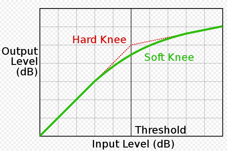
Some compressors also offer some control over what is called the “knee”, meaning the point where compression begins, above the threshold level. If the knee is “soft”, the compression is introduced smoothly in order to avoid an abrupt transition. A “hard knee” introduces the compression immediately once the threshold is surpassed, although in most cases this is inaudible.
There are at least two more standard variables in dynamic range controllers, the attack and release times (the latter sometimes being called the decay time, but it is better to restrict this term to the last portion of an amplitude envelope). The attack time refers to how quickly the gain control comes into effect (that is, the delay before compression or expansion starts), and the release time is how quickly that control is removed. These variables allow you to shape the gain control at the micro level of time.
Compression with "knee" control
To capture and control a sharp attack, you will need a fast attack time. This is usually stated in milliseconds (ms), or thousandths of a second, but it is not unreasonable with very sharp attacks, as discussed below, to need attack times in microseconds (µsec) or millionths of a second. Release times can go from a few milliseconds (very jerky) to a second or more (very sluggish) in terms of speed of response.
When you think more closely about it, the limiter has the most difficult job to do in this ensemble of dynamic range controls – it has to anticipate a level that may distort, and smoothly re-shape its level without audibly distorting the waveform in the process. In other words, a limiter that simply does peak clipping (i.e. a flattening of the waveform) is no limiter at all, or at least not a good one.
The limiter included in the professional Nagra recorders, as used by the World Soundscape Project in the 1970s, almost never had peak distortions called peak clipping (assuming that reasonable record levels were used). In an environmental situation, you can’t always do a “test run” rehearsal for setting levels if the event to be recorded is a one-time or unforeseeable occurrence.
In the analog world, the audio engineer could rely on the temporal behaviour of circuits, their latency if you will, that could be brought into play, but in the digital world it’s all numerical calculations, so what kind of algorithm could do the job effectively? This is beyond our scope, but in general, the limiter is restricted to recording and broadcast systems, whereas with audio mixes, compressors are usually used to keep the peak signals below the distortion level.
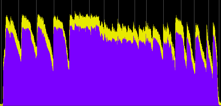
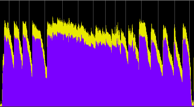
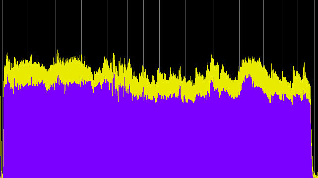
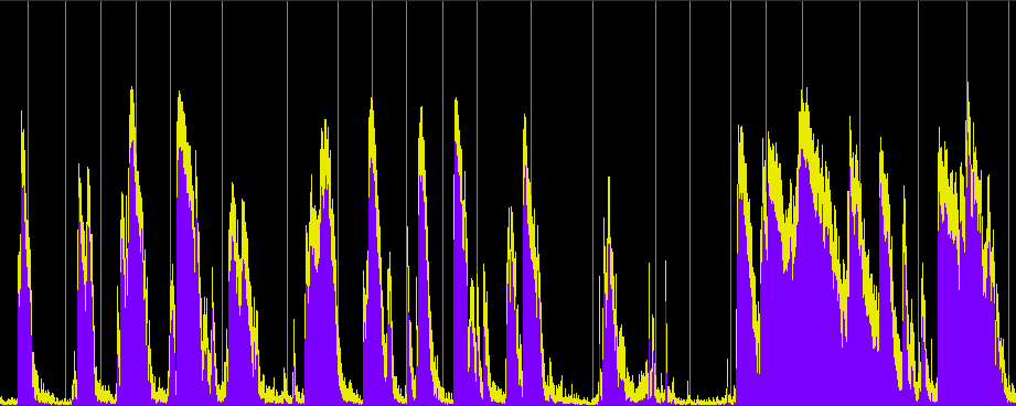
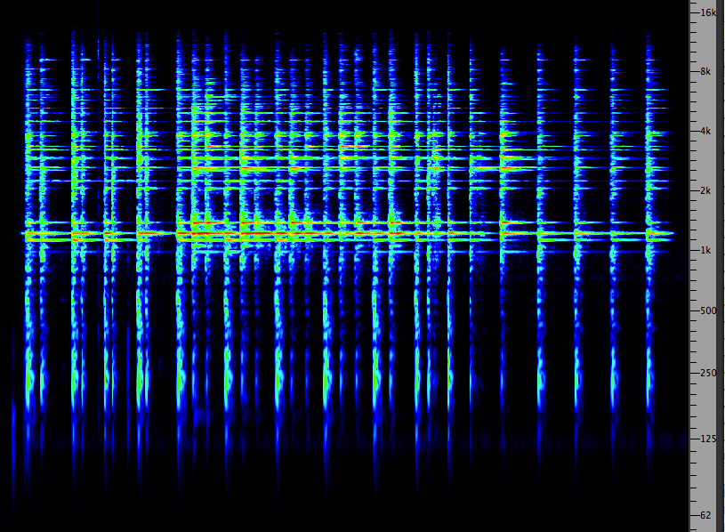
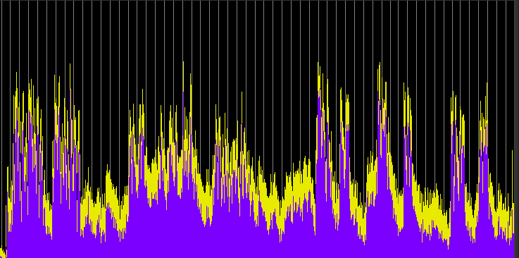
Examples of compression. In these examples we are going to use the Power Spectrum representation of our sounds to illustrate dynamic range control. The power spectrum is similar to an envelope display, such as produced by a graphic level recorder, but it actually represents what is called the root-mean-square (RMS) power which is the “real” or “effective” power, as distinct from a maximum amplitude display. We hope you won’t mind the hot colours of the display, but they somehow seem appropriate!
First we will hear the percussive sound of a German blacksmith pounding metal on metal, which is going to result in sharp attacks and a lot of high frequency energy in the 1-4 kHz range where the ear is most sensitive. Listening to a long sequence of this sound even at a reasonable listening level may get painful and cause a threshold shift in your hearing – dare we say a pounding headache?!
However, in terms of audio signal levels, like any percussive sound, the peak levels created may constrain how a mix is going to stay within the available dynamic range, and therefore how loud other sounds can be. So, for both of these reasons (audio and psychoacoustic) we may want to compress the signal.
These examples have two variables: (1) the compression ratio (using 5:1, 10:1 and 20:1), and (2) the threshold value where the compression begins, with two cases, namely -20 and -40 dB, which basically means just the high part of the signal level, or essentially the entire signal. Each processed sample has been given a 10 dB boost, with an attack of 1.2 ms and release time of 30 ms.
Original blacksmith recording
Source: WSP Eur 19 take 8
Power Spectrum (click any image to enlarge)
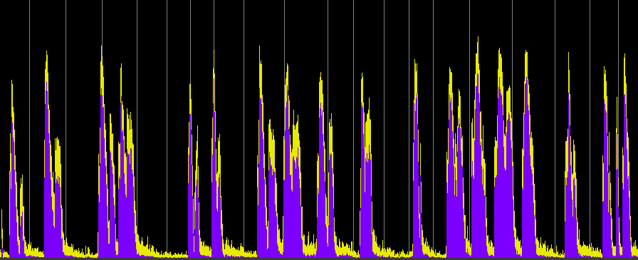
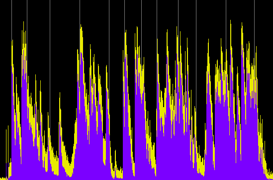
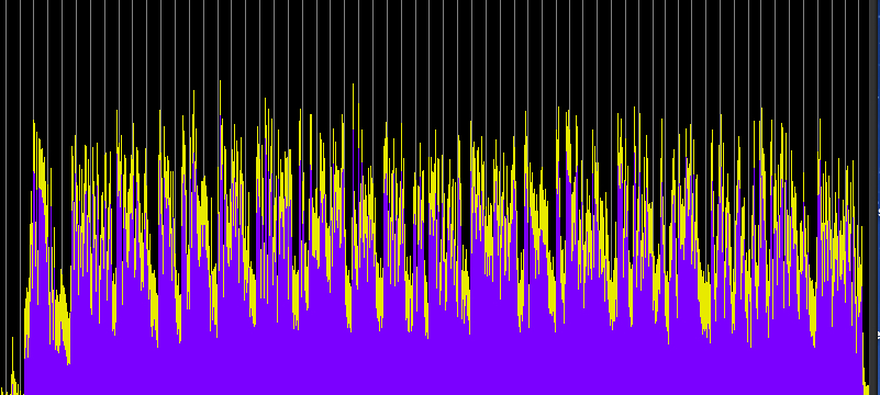
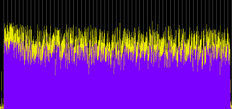
Compression ratio 5:1, threshold -20 dB
Compression ratio 10:1, threshold -20 dB
Compression ratio 20:1, threshold -20 dB
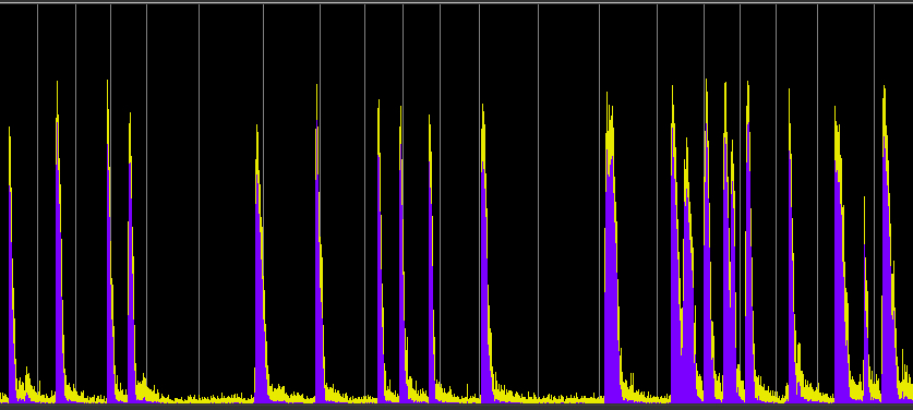
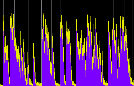
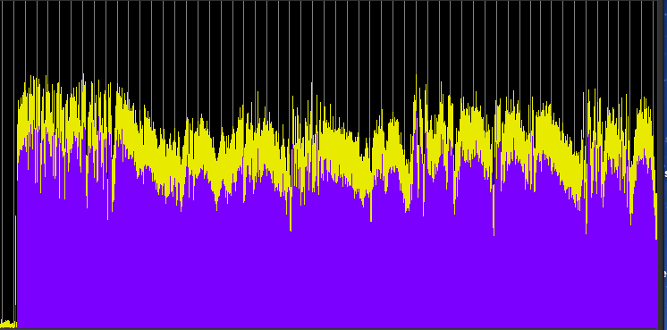
Compression ratio 5:1, threshold -40 dB
Compression ratio 10:1, threshold -40 dB
Compression ratio 20:1, threshold -40 dB
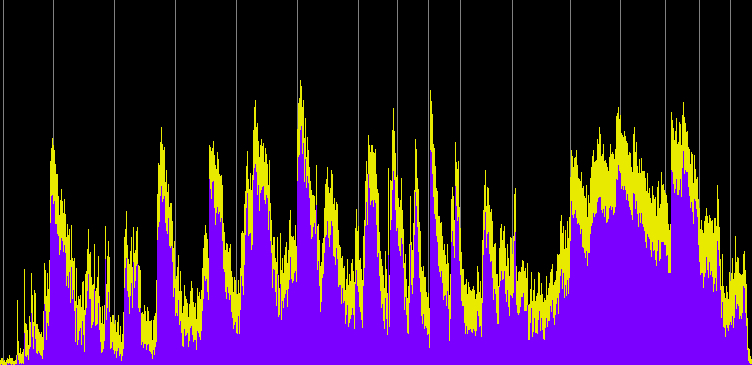
Compression ratio 20:1, threshold -40 dB and +20 dB boost
Compared with the well defined envelopes of the original recording, the first set of three compressions reduce and compress the envelopes of each hit, particularly during the middle section where the rings overlap. They now appear to have nearly constant levels (and therefore are louder). When the entire signal is compressed, then the overall level is drastically reduced, the hits become less well defined and almost ambient. We can still hear the differences in the spectrum, but in terms of loudness, the sound is levelled off to be almost continuous. The last example shows what happens when that level is boosted by another 20 dB and we lose all sense of temporal definition in the final rather emasculated sound.
Examples of Expansion and Gating. Here are examples of using an expander with different types of sound and intention. The first is an edited vocal text of percussive type words where an expander takes out any residual background noise (in this case, tape hiss) but leaves words such as “touch” intact. Then by raising the threshold about 10 dB, the sibilant consonants (such as “ch”) are also removed, leaving only the hard consonants.
In the second pair of examples, reverberation in a soundscape recording of locks and doors is removed by an analog expander with a fast attack and release time. The threshold was set just above the reverb level, so notice how the percussive sounds now “jump out” at you. Some EQ was also added.
In the third pair of examples, some percussive sounds with icicles are simply “cleaned up” by removing the low level bits of the sound, prior to what remains being subjected to further transformation.
Vocal consonants expanded, ratio, 1:10, threshold -25 dB
(Source: Norbert Ruebsaat)
Power Spectrum (click any image to enlarge)
Vocal consonants gated, ratio 1:10, threshold -15 dB
Locks and doors in reverberant environment
Locks and doors gated
Ice percussion
Ice percussion gated with plug-in
As useful as expansion is, as you can hear in the above examples, you should keep in mind that the low level sounds that are being eliminated in the pauses are still there during the sounds that are let through the gate. This is an analogous situation to filtering where there’s a clear distinction in frequency between the materials we want to keep, and those we want to reduce or eliminate. A filter with a relatively steep roll-off can be placed between those bands, but otherwise the filter cannot distinguish when the “desired” and “undesired” elements overlap in the spectrum. With expansion, we are making a similar distinction between low-level unwanted sound, and high-level sounds we want to keep, based on the optimal threshold level.
The traditional (but sometimes partial) solution to this problem, such as when you want to remove an unwanted drone or hum, is to use a parametric equalizer, such as a notch filter, to remove as much of the offending spectrum as possible, without compromising the foreground sound quality, and then add the expander or gate to remove its presence further during the quiet parts when it would be more noticeable.
Finally, we show the effect of attack time with compression on two shotgun blasts. These blasts have a rise time of about 10 ms, so if the attack time for the compression were set to that amount, the attack would be missed, and we couldn’t raise the overall level by 10 dB, which was done in the compressed examples. Each of these use much faster attack times of 1 ms, 100 µs and 10 µs. This allows compression with a modest 5:1 ratio to control the instantaneous peak levels and permits the 10 dB overall boost, thereby producing a much “fatter” sound.
Shotgun blasts
Source: WSP Can 1 take 11
Shotgun blasts compressed with 1 ms attack
Shotgun blasts compressed with 100 µs attack
Shotgun blasts compressed with 10 µs attack
Frequency dependent compression. Given that compression has traditionally been used in radio broadcasting, a specific case of needing to compress a particular frequency band began there. This was in reference to reducing the brightness of the high frequency consonants known as sibilants (the narrow-band noise based consonants such as ss, sh, ch, or their voiced versions - see the Speech Acoustics module). These speech sounds became more prominent on radio because voices were being close miked, and therefore these high frequencies went straight into the microphone and were found to be annoying to listen to if they were particularly strong in certain voices.
The process of reducing these frequency bands (5 - 10 kHz) is called de-essing, and can be achieved in a variety of ways, some of which are available in plug-ins. This example is with a vocal text chosen for its sibilants, which towards the end are exaggerated. In other words, the original intent was to capture these sounds (and process them), not reduce them, but for the purpose of demonstration, we will do that. In this case, a simple filter roll-off would have achieved about the same result, but it does show that this upper frequency band can be compressed independent of the rest of the spectrum.
Voice with sibilants
Source: Norbert Ruebsaat
Same voice de-essed
spectrogram at right
Click to enlarge
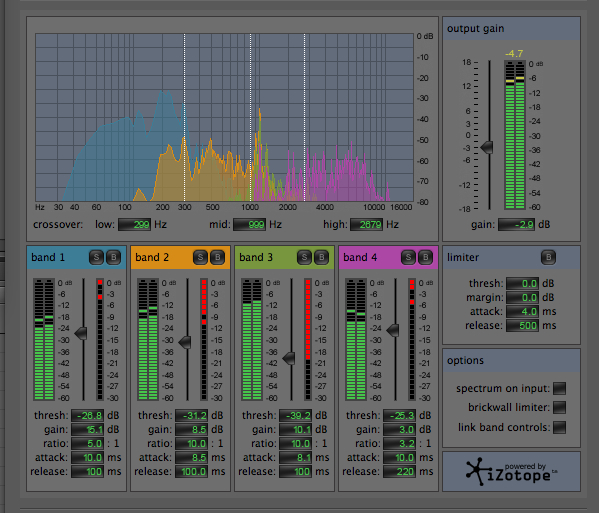
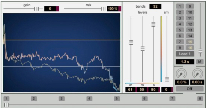
Today, multi-band compression, while computationally more complex, is a powerful tool for re-shaping the spectral balance of any sound. However, as stated earlier, in order to use it effectively, you need to understand the compression model and its parameters as outlined above. Where de-essing involves only a single band, assumed to be in the high frequencies, a multi-band compressor spans the entire range and divides it into a number of separately controllable frequency bands.
This colour-coded four-band compressor in Audition provides an excellent interface for doing that, but again, note that you need to manipulate the parameters directly, without seeing the straight-line representation of the process.
Using this processor is also a good listening exercise, because there is a “solo” button next to the number of each band, thereby allowing you to hear your detailed adjustments in real-time for just that band. The crossovers between bands are adjustable in the top diagram, as indicated by vertical lines above the spectrum in question. These overlaps are useful in order to keep the processing smooth.
Multi-band compressor in Audition
The graphic levels for each band (green for input and red descending lines to show the amount of compression) are helpful for seeing what is happening as you listen. The threshold value for each band can be adjusted in reference to the signal level, and the other four parameters can be typed in or dragged up or down. It is best to solo each band while adjusting them, then add in one or more other bands for previewing the end result.
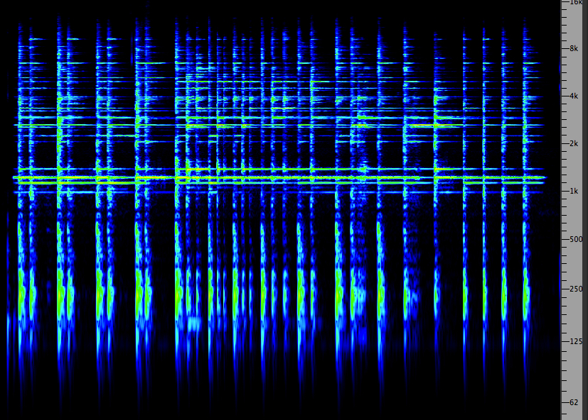
Here we use the blacksmith soundfile again, as above, but instead of just compressing the peaks or the entire signal as we did earlier, here is a more elegant and effective way of changing the percussive envelopes and the associated spectrum with the purpose of (a) making the attacks less intrusive and tiring to listen to and (b) emphasizing the percussive lows, while keeping the upper resonances more sustained. The parameters used are the ones in the above interface diagram.
Blacksmith
Blacksmith with multi-band compression
Click to enlarge images
Spectrogram of original recording
Power spectrum after multi-band compression
Spectrogram after multi-band compression
Note that the multi-band compression used here keeps the individual strikes better defined than did simple compression shown above in the power spectrum. In terms of the frequency spectrum, the lows now are given more “bite” and prominence, and the overly strong frequencies around 1 kHz are toned down and evened out with the upper partials to form a more pleasing balance of resonances.
The compression/expansion concept and its parameters are becoming a standard approach to spectral design, as shown here with the multi-band compressor, but also with other apps such as SoundHack’s Spectral Shapers, or GRM Tools’ Contrast, each with its own unique interface and controls. Therefore it is advisable to become familiar with the concepts outlined in this module as they have increasing applicability in the spectral domain.
GRM Tools Contrast, with a re-balancing mix of weak, medium and strong frequency ranges
Index
C. Historical uses of compression in broadcast and recording media. Compression and limiting were initially developed as a solution for some practical problems in broadcasting. First, a limiter was needed to prevent potentially damaging peaks levels from overloading the equipment, including the transmitter, and this type of protective circuit is often incorporated today into a range of other equipment for the same purpose.
As we have seen and heard, compressing a signal allows it to not only avoid distortion (called over-modulation in radio) but also to make it sound louder. In the early days, making the signal sound louder also meant it sounding more clearly at a distance against radio static, for instance, and in noisier situations like automobile driving as well as on the cheaper speakers used for radio reception. All of these reasons combined to enhance the economic potential of reaching a larger (and more mobile) audience. And, as a result, compressed audio became synonymous with radio.
Similarly, recordings benefited from compression and limiting, particularly as more full-bandwidth sounds were being cut into the grooves of a long-play record. The limiter prevented damage to the equipment, and compression produced a better signal-to-noise ratio for the recorded sound compared to the surface noise of the record itself.
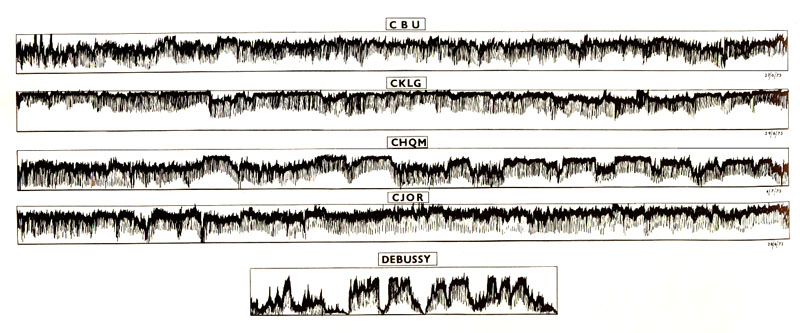
In the 1950s and 60s, as radio formats became designed for specific target audiences, not only did the content change (the type of music, announcers and ads), but so did the use of compression. Foreground pop music stations compressed their signals to ride high in the overall dynamic range, whereas background music stations did the opposite. This comparison of an hour broadcast from four Vancouver AM stations in 1972-73 was typical. All were designed in different ways to be an “accompaniment environment” – a soundscape in fact – for listeners involved in other tasks.
The pop music station (CKLG), playing already compressed records, compressed them again with smoothly overlapping announcements and ads, and rode their signals to be as loud as possible. The background music station (CHQM) was less intrusive with a medium level of compression and slower transitions, essentially providing a non-demanding ambience. The talk radio station (CJOR) had a larger dynamic range because of the predominance of voices, and the public broadcaster (CBU) did the same with a mix of music and voice.
Comparison of the dynamic contours of four Vancouver AM stations over one hour, early 1970s.
Source: Vancouver Soundscape document, 1973.
For comparison, a graphic envelope of a piece of symphonic music by Debussy is shown with a much larger dynamic range. Of course, this type of music, with its quiet passages, was harder to listen to in a car because of the motor and tire noise present, so in practice, most listeners came to prefer the sound of compressed music.
During this same period, ads on television were often regarded as being louder than the program material because of their enhanced compression and the fact that they were more likely to be surrounded by pauses. Federal legislation limited the level of broadcast signals, so advertisers resorted to greater compression in order to stay within those guidelines but still compete for attention via loudness.
Ads on radio took the opposite approach. Since the surrounding program content, particularly recorded music, was already highly compressed and therefore produced a habituating effect on the listener with its near constant loudness, the commercial breaks actually expanded the dynamic range of the signal in order to draw attention. Key to making this transition as smooth (and unobtrusive) as possible, was the role of the announcer who would lead the listener out of the previous music track, for instance, by giving seemingly useful information and then transitioning directly into an ad sequence.
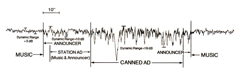
Manipulation of dynamic range during a commercial break on a pop music station, 1970s
Source: Truax, Acoustic Communication, chapter 11, 2001
This diagram shows such a tight sequence on a popular music station in Vancouver in the 1970s. The dynamic range of the music is measured at 5 dB, and since it’s a foreground format station, the announcer talks over the end of the song and moves the listener’s attention seamlessly into a “station ad” (or “announcer ad”) promoting a local concert (and obviously crudely put together). This sequence enlarges the dynamic range to about 10 dB, and then without a millisecond of a break there is a sharp cut to the major canned ad in the sequence that is attention getting, partly because of its highly crafted sounds, its compelling narrative, electronic effects suggesting the thrill of skiing and – most amazingly – an actual moment of silence in the middle of the ad at a dramatic point in the narrative. The dynamic range for this ad is doubled again to 19 dB (not counting the pause), at the end of which the announcer is cued to speak over its conclusion and quickly leads the listener back to the next bit of music.
In today’s digital broadcasting studio, such precision of synchronization would be produced by a computer program, but at that time, the 1970s, it was all done by a disc jockey manipulating the source tracks and doing the commentary and cueing. The effect was to allow the paid ad to surface into the listener’s consciousness, and in this case, to appeal to a latent desire to get away from the city and take some ski lessons as an adventure, just as the ad itself as an audio experience brought new energy and emotional excitement into an otherwise predictable wall of music.
Although the specifics of ad breaks on this foreground format differed from all of the other three formats diagrammed above, they were all variations of a similar theme of providing a predictable accompaniment soundscape. A predictable program structure was designed to hold the listener’s attention through its continuity, and provoke potential interest in the products and services being advertised through a manipulation of dynamic range.
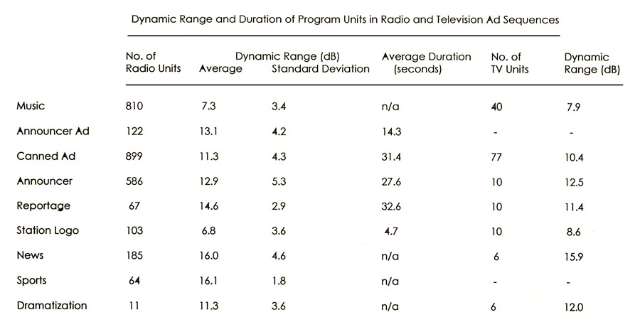
In a survey of 10 Vancouver radio stations in 1991, representing all available formats, including foreground and background stations, 785 program segments such as the one we just presented, were analyzed along with over 2800 program elements of all kinds, along with their duration and dynamic range, as shown in this table.
The average dynamic range for all music segments was 7.3 dB, and both types of ads (announcer and canned) had dynamic ranges of 11 to 13 dB. Voice segments, of course, had a higher dynamic range. The chart also shows a similar analysis of 6 hours of a music video TV channel from 1992 that revealed its similarities in format and structure to its radio counterpart. The canned ads also had a higher dynamic range than the music.
Analysis of radio and TV program elements according to dynamic range
Source: Truax, Acoustic Communication, chapter 11, 2001
Our conclusion was that dynamic range played an important role in guiding listeners’ attention, particularly within the context of an accompaniment medium where program content largely stays at a background attention level, and ads had the potential to lift that attention level during the ad breaks. Since listeners have the option of changing stations or channels with just a button, maintaining a smooth continuity of predictable program segments (without jarring louder segments) was needed to hold the listener’s attention.
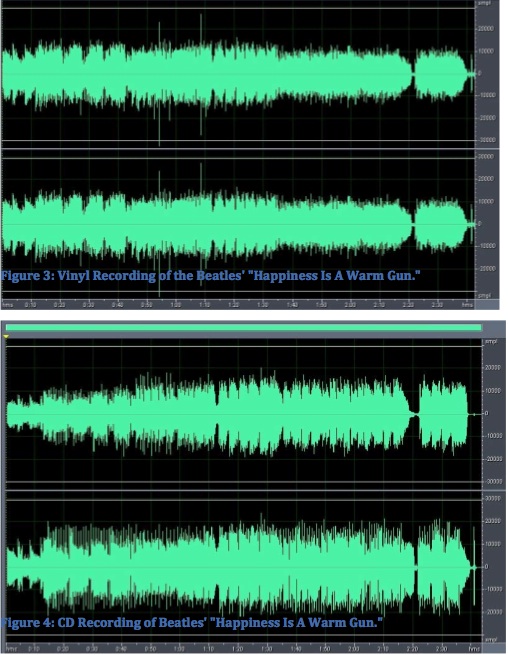
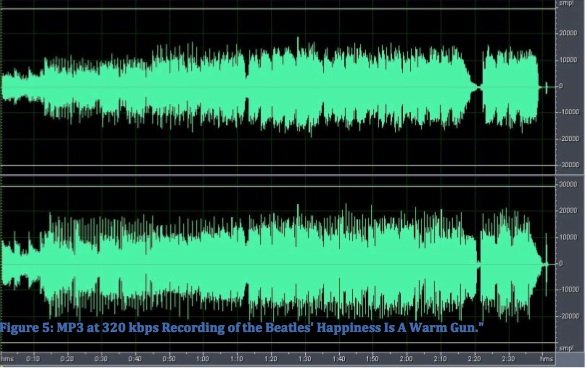
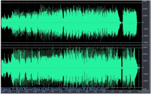
The commercial recording industry has increasingly used high levels of compression to make their recordings sound louder, to the point where there has been strong criticism of the practice referred to as the “loudness wars”. There are many examples of this trend as can be seen on the Wikipedia entries for “dynamic range” and “loudness wars”. Re-mastering of the same material in different time periods has been a simple way to illustrate the phenomenon, such as these examples for a Beatles song, including a comparison of the original vinyl version with the CD, an mp3 version, and a more recently re-mastered version, each showing a greater use of compression.
Beatles vinyl compared to CD
Beatles mp3
Beatles re-mastered
Dynamic range comparison of a Beatles song in different formats
Index
D. Examples of bad compression. If the effects of compression become obvious (and aurally annoying), then it is not being done properly. On the other hand, listeners generally seem to be less sensitive to the manipulation of dynamic range than they are to, for instance, poor frequency response or obvious signal distortion. It is difficult to determine whether it is because compressed signals are the norm on radio and recordings, and therefore familiar, or whether we become used to loudness being relative due to our own constantly changing threshold shifts in different sound environments – or maybe both.
Obvious examples of bad compression are when a strong sound causes the loudness of weaker sounds that are present to change their own loudness level, an effect called pumping. Of course, there are often creative uses of artifacts, such as in dance music where the pumping is synchronized with the beat. However, in other cases, the effect is distracting and seemingly unnecessary.
Environmental sounds, with their potentially much larger dynamic range when recorded outdoors, become difficult to broadcast on radio if automated compression is being used, as it usually is. Here is an egregious example of a broadcast on the CBC Ideas program in 2017 where Hildegard Westerkamp took a CBC announcer on various soundwalks that included live commentary between them.
The Ideas program’s usual content is a close miked voice speaking from an acoustically controlled studio similar to a formal lecture without the need to project the voice. A compression technique known as upward compression is sometimes used in case the speaker’s voice drops a bit, or is momentarily “off mike”. This kind of compression raises low level sounds back to normal level, as shown here.
Upward compression
Unfortunately, in this program, there were many lower level environmental sounds, which were the actual subject of the program, but because of upward compression, they suddenly jumped out as if they were close by, hence ruining the effect of the soundwalk and interfering with the commentary going on. In the last example, the commentators were briefly off-mike on their walk at Kits Beach and in fact a bit harder to hear, so the technique might have helped a bit then, but for the rest of the program, it completely ruined the aural experience.
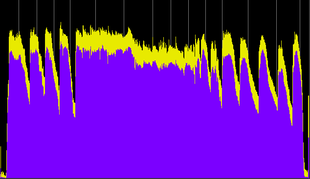
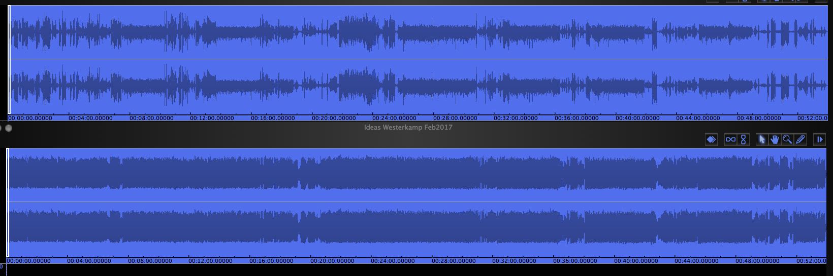
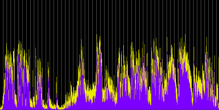
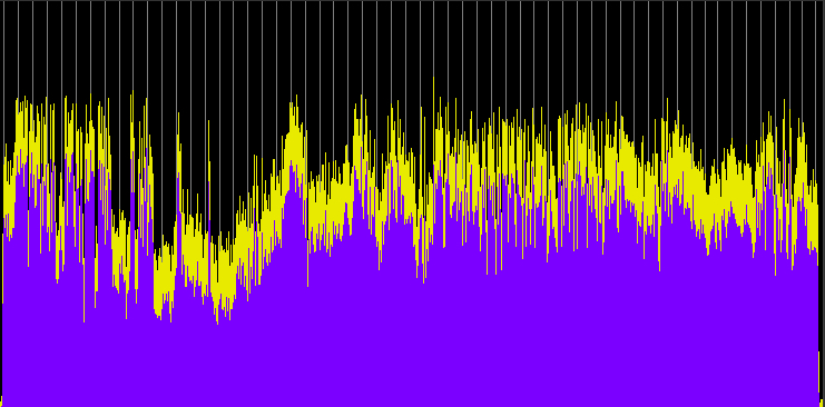
First we’ll show an overview of the dynamics of the entire broadcast, in comparison with the online version which thankfully escaped compression and was identical to the original mix. Also fortunate was that when the World Soundscape Project's Soundscapes of Canada was broadcast on the CBC in 1974, the program was in stereo and this kind of compression was not used.
Dynamic range comparison of the original (and online) version of CBC Ideas soundwalking program with Hildegard Westerkamp (top), and its actual broadcast version (bottom). (click to enlarge)
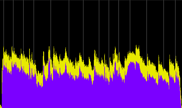
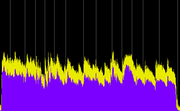
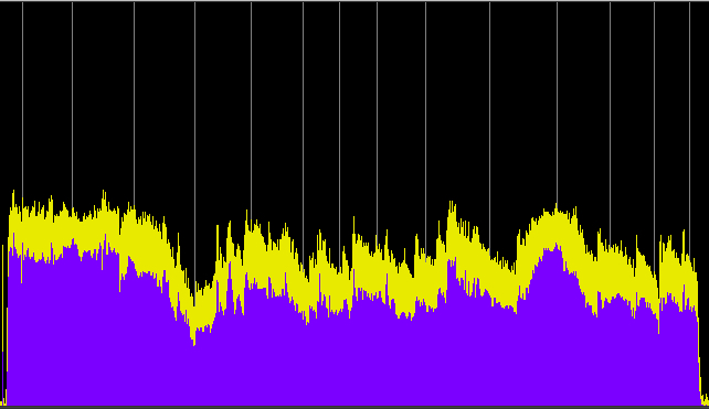
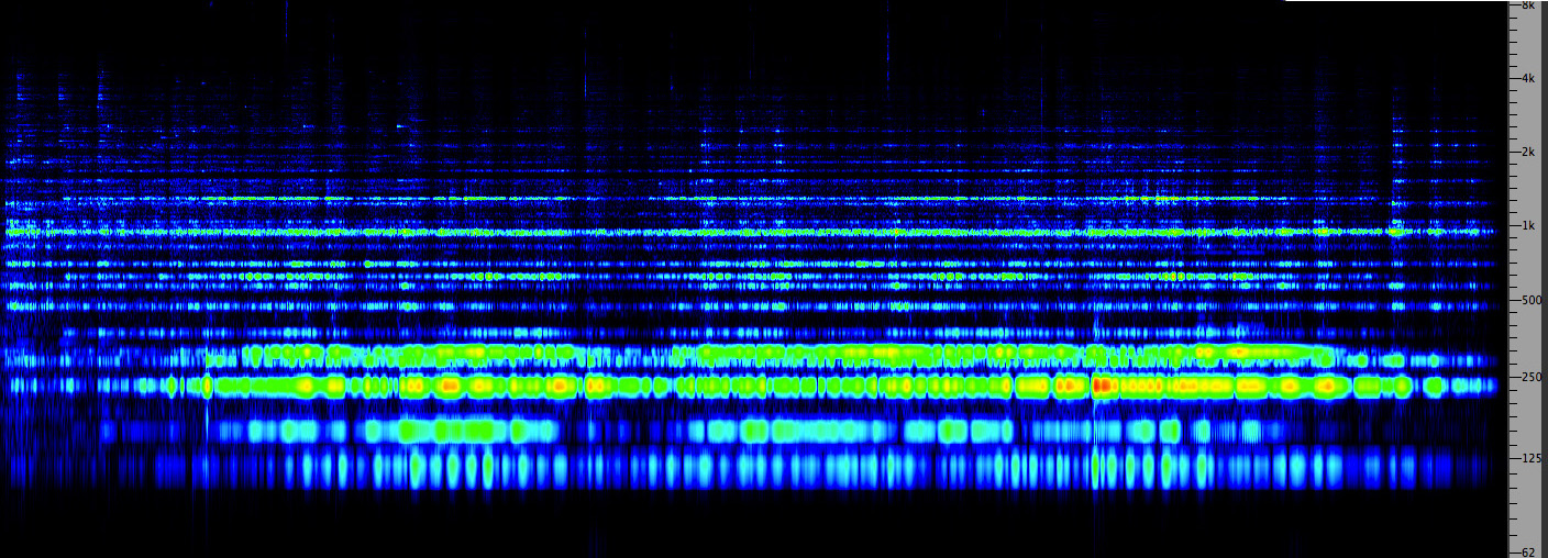
Next, we will compare three segments of the original program with their broadcast counterparts and the associated power spectra. Warning: the broadcast segments are painful to listen to!
Ideas excerpt original, 11 min.
Ideas excerpt as broadcast
Ideas excerpt original, 22 min.
Ideas excerpt as broadcast
Ideas excerpt original 31 min.
Kits Beach sequence
Ideas excerpt as broadcast
Three excerpts of CBC Ideas program on soundwalking with Hildegard Westerkamp, comparing the original to the compressed broadcast version in 2017.
Index
E. Studio demo’s of dynamic range control. In the above sections, we have already provided examples of common approaches to dynamic range control, namely compression, expansion and gating, and multi-band compressors. Here we will discuss some other issues about these processes.
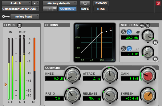
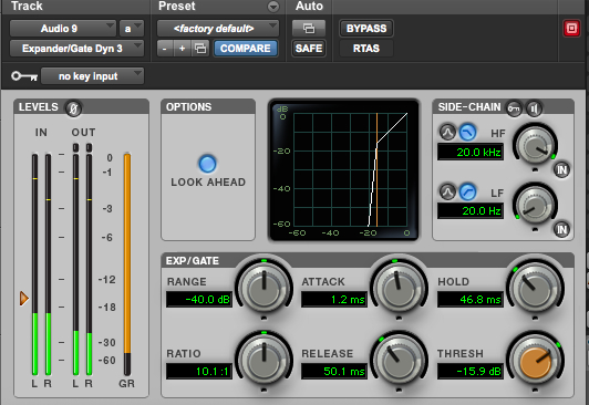
First of all, it may be useful to compare some typical interfaces for these processes. As already pointed out, the dominant model is either a parameter group illustrated by the typical input/output response diagram we have used to understand the process (as in ProTools), or its variant, a direct graphic control over those values with the corresponding numerical values indicated (Audition example). Some simpler interfaces are just a bank of numerical values for each parameter, in which case you really need to know what those numbers mean. Let’s start with some compression interfaces.
Pro Tools compressor
Note the input and output levels (green) at the left besides the compression level (orange) working in real-time.
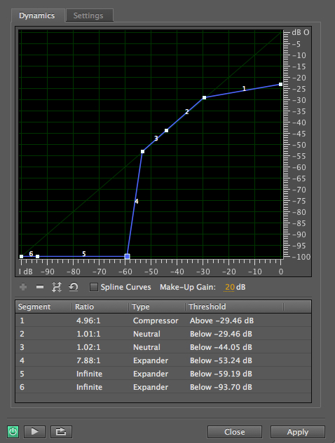
Audition compressor and expander combined
As you can see, Audition’s compressor (right) allows you to build the response diagram yourself as a set of up to 6 line segments, with the corresponding process and numerical values indicated below it. In this case, line 1 indicates the compression ratio (5:1) above a threshold of about -30 dB, and line 4 is an expander ratio of about 8:1 (which should read 1:8) below -53 dB, with a linear range in between. A make-up gain (that is, a signal boost) is also specified. Although the processing can be controlled interactively with the sound, there is no indication of how the signal levels are being processed, as in ProTools.
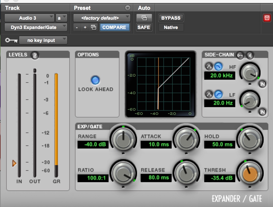
Next we show ProTools’ Expander and Gate, which are really the same interface, except the gate ratio is set to the maximum value.
ProTools Expander with a high threshold
ProTools Gate with a low threshold
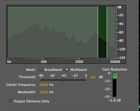
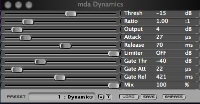
Here are two other simple interfaces, the first for de-essing, where the bandwidth and compression ratio is specified, with a graphic representation, and the second is the simple mda gate which also has numerical compression values (that are neutralized by setting the ratio to 1:1) and the gate is activated with a threshold of -40 dB. This was the plug-in used for the icicle percussion example above. Gating is not a process that really needs a sophisticated interface as the threshold is the main parameter.
Audition de-esser showing gain reduction in the highs
mda compressor and gate
Secondly, and more importantly is the issue of when to use a compressor in the first place. The two contexts are (a) to modify a particular soundfile and (b) to apply compression to a mix.
All of the examples in section A of this module were chosen to show you some options for modifying an individual soundfile, with the implication that you would fine tune the parameters for a particular sound (and possibly save the values as a preset if that is allowed), apply the process to the sound and save it as a new soundfile that could be used in a mix.
In other words, it doesn’t make much sense to do this in a mix, probably because this type of processing is designed for only a certain sound, and is unlikely you’d want to apply it to anything else. It is also likely you can do a better job of detailed sound design on your sound in such an independent manner.
Moreover, a sophisticated process like the multi-band compressor is computationally very expensive, and it could take up too much processing capability during a mix so it is best done beforehand. Such a processed sound could also be further processed into other variants, or transpositions, or more complex processing, such as time stretching or convolution.
Keep in mind that if your editor doesn’t have a good dynamics processor, you can always set up a small, dedicated multi-track session just for this process, and perhaps use it later for other similar situations.
Compressing a mix (or not). Next we come to the use of compression in a mix. There are several typical contexts here as well:
(1) you have a percussive sound with lots of peaks that are making it difficult to combine with other sounds in the mix, orIn this last case, then the only solution is put a stereo compressor on the master output channels and let it affect everything in the mix.
(2) you are mixing down a multi-track session to stereo, for instance 8 to 2 where four tracks are being combined into one, or
(3) you need the entire mix compressed for use in, for instance, a video or film soundtrack that is unlikely to have a large dynamic range.
Why not do the same for the first case? The answer is another question: why compress other sounds in the mix when there’s only one or maybe two tracks that need it? It would probably make more sense, and be safer in some sense, to put the compressor just on the tracks with the problematic file with all the peaks – or do it previously in an editor with a compressor plug-in.
There is also another, more detailed way to avoid using a compressor at all in a mix, and that is the tradition of “riding the levels” manually. In the analog world, all mixes were interactive in real time, and so mixers were set up to allow you to use all of your fingers to control levels simultaneously, and most importantly, in reaction to what you were hearing.
Unless you have a digitally controlled mixer, you have to latch levels in your mix and control them with a mouse. It is good to do that in a DAW with every track of the mix, but for now let’s stick with the problem of keeping peak levels below saturation.
Here is a simple example. In my piece Earth & Steel (2013), the main source material are the hits on a metal ship hull, the same one used to illustrate volume in previous examples. Each hit is also auto-convolved several times to lengthen the sound and create an even greater spectral richness when combined in a multi-channel format (in this case 8). During the first 5’ of the piece, the hits build up to a dramatic percussive peak with 3 hits followed by 7.
Given the multi-channel format, the acoustic energy is spread out over 8 channels (an effective alternative to raising the amplitude on a single channel) and therefore no compression was needed, at least not until the climax with the major 3-7 hit. Would it be worth compressing this peak? Perhaps, but the alternative solution was simply to ride the levels and record them via latching, as shown in the excerpt from the ProTools session showing the lowered amplitude levels. This alternative form of compression could be rehearsed and modified to keep the overall signal under the maximum.
Percussive peak
Earth & Steel
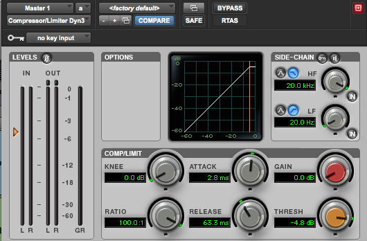
Riding the levels during the peak
ProTools limiter (click to enlarge)
However, during the eventual mixdown to stereo, a limiter (as shown at right) was inserted on the master track just to be on the safe side, as shown, but the master track levels were also modified interactively during the peaks, although admittedly a compressor could have been used on the entire process.
Refining levels in a mix. As remarked previously, it is surprising that given the expanded dynamic range of digital audio, where a 24-bit mix is arguably the standard, that this dynamic range is not better and more fully used. It would be easy to argue that the single biggest flaw in digital mixes is a lack of dynamic variety in sound levels. Whether this is the result of hearing so much compressed music elsewhere, as documented in section C, or the move away from physical mixing consoles, is debatable, but the result is the same – uniform (and very boring) loudness levels.
Listeners are accustomed in the acoustic world to relating effort with spectral richness and hence loudness, and not merely absolute sound level (to which our hearing adapts anyway). Purely digitally processed sound is not constrained by physical effort or gesture, and therefore it is easy to have a disconnect between the apparent loudness of a sound and the “energy” that it implies. Of course, this connection can be restored during a diffusion style performance of the track in an actual listening space, but will something similar be communicated by listening to the track without that type of interpretation?
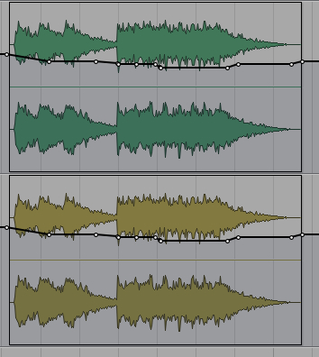
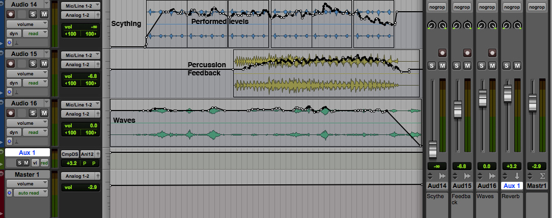
In the previous Reverberation module, we constructed a mix of disparate elements (scything, waves, and percussive sounds with feedback) unifying them with medium reverberation. Here we return to that example and add levels interactively using the Latch and Touch functions with each of the three stereo tracks as shown here.
Original mix
(click any image to enlarge)
Spectrogram of original mix
Mix with adjusted levels
Spectrogram of mix with adjusted levels
The scything track, which was rather uniform in loudness, now has a contour added with peaks and valleys, the peaks meant to coincide with the larger waves which are also increasingly exaggerated. These levels were modified using “Touch” so that the previous levels could simply be amended with those peaks. The percussive track in Latch mode now starts out at a lower level and builds, with increasingly energetic peaks in synch with the beat that emerges.
The waves + scything now reach their own peak, followed a few seconds later by the percussive peak. Luckily the mix stays within the available dynamic range with only a 3 dB reduction on the master level, and leaves just .8 dB to spare in terms of headroom, so there is no need to normalize the mix (see below). The overall mix now has more intricate interactions between its components and two well-defined peak moments.
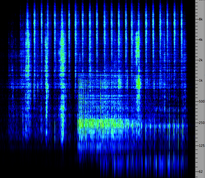
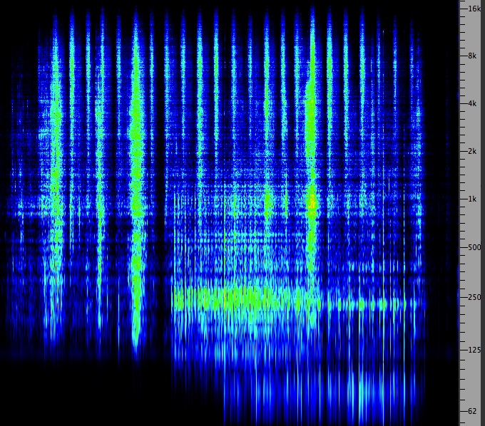
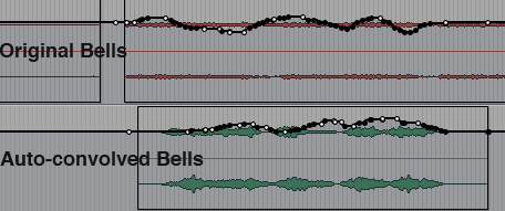
Here is an example of a more subtle mix between realistic and processed elements that attempts to blend them smoothly enough that the listener can seem to go "inside" the sound itself, as if in a daydream. The excerpt is from my Bells of Salzburg (2018) near the beginning where I cross-fade a pair of bells with their auto-convolved version, which of course has the same spectrum, but with the attacks smoothed out.
The diagram shows the mixing levels that go in opposite and complementary directions – when the original track decreases, the auto-convolved one increases, in each of the three long “waves” by 4, 5 and then 6 dB until they finally return to the normal level of the original over a two minute duration.
Excerpt from The Bells of Salzburg
Click to enlarge
Normalization. At this point we should distinguish the above issues from the standard practice of normalization. The peak levels in a mix should be kept to slightly below the maximum possible values within the dynamic range of the medium. The process of raising all levels to this optimum point is called normalization, and you may have an automated option for that on your editor.
However, the software may also provide an analysis of peak levels as part of the file metadata, at which point you can globally add a certain dB level to bring it up to at most .5 to .2 dB below saturation, although many producers would prefer 1.5 dB. Sometimes this is expressed as a percentage, such as 99%.
This type of normalization only refers to the signal itself and its peaks. Today, with many different digital media formats available, including streaming, there is a move towards Loudness Normalization, using the LUFS method (Loudness Units relative to Full Scale) which allows similar programs, such as podcasts or videos, to have comparable levels of perceived loudness according to an international standard for loudness scaling.
One value of normalizing a track, besides ensuring that there is no peak clipping, is to make the mix comparable in overall loudness to other material that may surround it, or to simply reflect a typical listening level. Listeners have preferred monitoring levels for specific types of audio listening, and so if your track sounds weak, they will have no option (other than skipping it) but to increase the monitoring level, which might also be dangerous if there is a sudden peak.
Of course, you may actually want to create a uniformly quiet mix, and so it would defeat the purpose to normalize it. So, the final criterion also needs to be to match the implied volume and energy of the component sounds in your mix to the desired playback level. Although it may seem entirely subjective, you’re more likely to find agreement between listeners as to what the “natural” or appropriate playback level for a given soundtrack should be. In fact, it’s hard to listen to a mix attentively if it seems too weak or too strong.
You also need to consider your own level of hearing loss and have it checked periodically. As documented in the Audiology module, most noise-induced hearing loss is centred around a 4 kHz notch, which increasing spreads around that frequency with repeated exposure. Someone with a severe impairment in this region will tend to equalize their mix to be overly bright, if not intensely annoying to someone with better hearing. In that case, it is advisable to check your mix with someone with better hearing so that you’re not over-compensating for your own loss.
Index
Q. Try this review quiz to test your comprehension of the above material, and perhaps to clarify some distinctions you may have missed.
home